Modeling Workflows
1. Overview
Each section of this chapter is an ordered sequence of steps for one kind of project, with a link at each step to the chapter that covers it. The workflows share one model file: a building started in §2 can take on HVAC alternatives (§4), an EEM study (§5), a calibration (§6), and a PRM baseline (§7) as the project develops (What Is EP3?).
2. A new building, from the Model Wizard to results
- Start the model. File > New opens the Model Wizard. On Model Settings, choose the units, the weather file, the climate zone, and the run period (The Model Wizard). A new model sizes from extreme periods of the weather file; add ASHRAE design days when the project sizes to them (Weather, Climate, and Design Conditions).
- Pick the templates. Check the space types, the construction set, a service hot water system, and one or more HVAC systems. Each HVAC system becomes an EEM (The Model Wizard).
- Choose the geometry method. On Building Geometry, choose I want to draw my own building geometry for a real building. For a quick test of a system or template, Let EP3 draw a rectangular building for me gives a perimeter/core box that can be simulated straight after the Wizard (The Model Wizard). Click Execute Wizard.
- Draw the building. Add floors, trace the spaces over background drawings of the floor plans, let the walls and roofs follow in Automatic mode (the default for a new model; in Manual mode, generate them yourself), and add windows (Creating Building Geometry).
- Zone the building and assign templates. Group spaces into zones where the design’s zoning calls for it (Spaces and Zones), and check that each space and zone has its
SpaceTypeandZoneType(Internal Loads, Space Types, and Zone Types). - Refine the inputs where the design departs from the templates: constructions (Constructions and Materials), windows and shading (Windows, Shading, and Daylighting), loads (Internal Loads, Space Types, and Zone Types), and schedules (Schedules).
- Finish the HVAC. Adjust the template system, or build one from components (The HVAC Outliner and Creating HVAC Systems). Check which equipment serves each zone with View Zone HVAC Assignments (Zone-Level HVAC Equipment and Zone Sizing).
- Add tariffs if the results need energy cost (Utility Costs).
- Validate. Click Validate and fix what the Model Validation dialog reports (Model Troubleshooting and Quality Assurance).
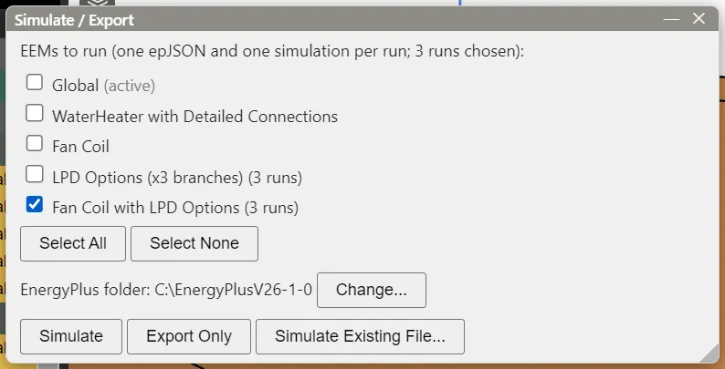
- Simulate. Click Simulate, check the EEMs to run in Simulate / Export, and choose a folder (Running Simulations).
- Review the results. Click View Results. Check the Unmet Hours tab before reading energy use, and the HVAC Sizing Summary for the design loads (Viewing and Interpreting Results, Heating and Cooling Loads).
As the design develops, edit the same model and run it again, with design alternatives as EEMs (§5).
3. A model from an EnergyPlus file
3.1 One IDF or epJSON file
- Open a blank model. File > New, then Skip - detailed mode in the Wizard. To add the file to an existing model, skip this step.
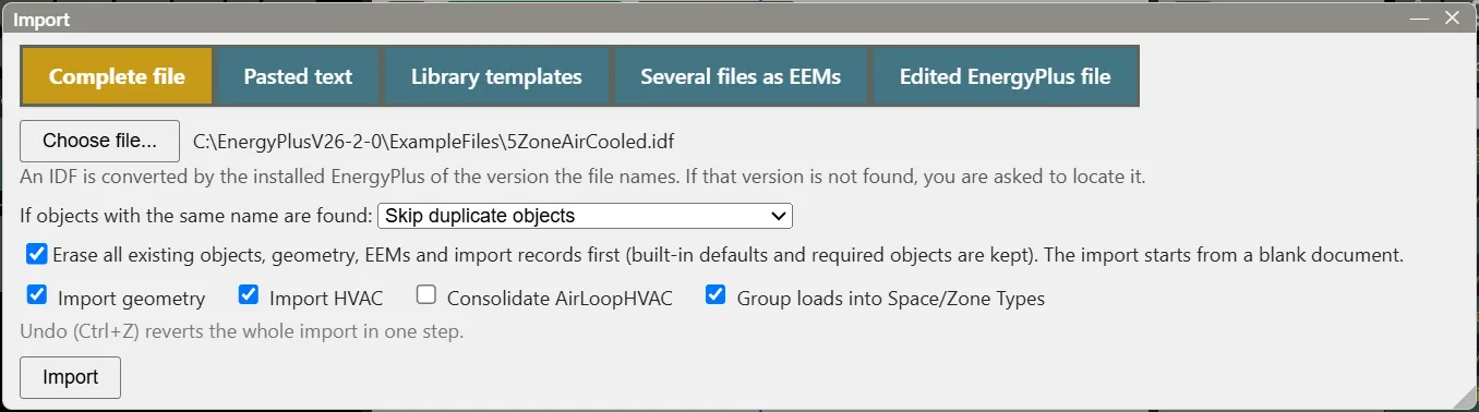
- Import the file. Click Import, open the Complete file tab, and pick the file. Choose whether to bring in its geometry and HVAC (Import geometry, Import HVAC), whether to merge air loops that are the same system serving different zones (Consolidate AirLoopHVAC), and whether to turn its loads into templates afterwards (Group loads into Space/Zone Types, which opens the Combine dialog when the import is done) (Importing EnergyPlus Files, Internal Loads, Space Types, and Zone Types).
- Read the import report in Model Settings > Import Details, and the objects that did not come in as they were in the file under Import Errors Summary (The EP3 Interface and Model Settings).
- Set the weather file, which an EnergyPlus input file does not name (Weather, Climate, and Design Conditions), and the climate zone if a PRM baseline will follow (§7).
- Validate, simulate, and review as in §2, steps 9 to 11.
3.2 Several variant files
When several EnergyPlus files are variants of one building, such as a baseline and its design options, Several files as EEMs makes them one model. It replaces the current model and its EEMs (unless Erase all is turned off).
-
Click Import, choose Several files as EEMs, click Choose folder… for the folder that holds the files, and tick them (Filter, Select All and Select None help with a long list).
-
Check the proposed structure: the root file supplies Global’s values, and every file becomes an EEM that stores only what it changes, built on the files whose changes it also makes. Change the root or a file’s parent where needed, and check Alternative: a file with another HVAC or SWH system is proposed as an HVAC or SWH System alternative.
-
Click Zip into one model. Global is left out of Simulate; each file’s EEM simulates as that file. Continue with the EEM study in §5.
Importing EnergyPlus Files covers the options.
3.3 Edits made outside EP3
To edit an exported file in a text editor or another tool and bring the edits back:
- File > Export epJSON… writes the EEM’s epJSON.
- Edit the file.
- Click Import, choose Edited EnergyPlus file, and pick the file (IDF or epJSON). Exported from: names the EEM it came from, beside a count of the objects changed, added, and removed.
- Choose where the changes go: A new EEM (built on the EEM of your choice), Into the EEM, or Into Global, and click Merge changes. What could not be brought back is listed under Not brought back:.
4. Comparing HVAC system alternatives
- Bring in the candidate systems. Check them together on the Wizard’s HVAC Systems tab (The Model Wizard), or add them later with Import > Library templates (The Model Wizard). Each system becomes an EEM with Alternative Category HVAC System (The HVAC Outliner and Creating HVAC Systems). §4 of that chapter covers choosing between zone equipment and air loop systems.
- Build a system the library lacks. Add an EEM, set its Alternative Category to HVAC System, and select it in the EEM dropdown. Everything added to the HVAC side while it is active is on only in that EEM (Energy Efficiency Measures (EEMs)). Build the system (The HVAC Outliner and Creating HVAC Systems) and assign its zone equipment with View Zone HVAC Assignments while the EEM is still active.
- Vary one system (a higher fan efficiency, a different chiller) in an EEM built on that system’s EEM, with Alternative Category left at None (Energy Efficiency Measures (EEMs)).
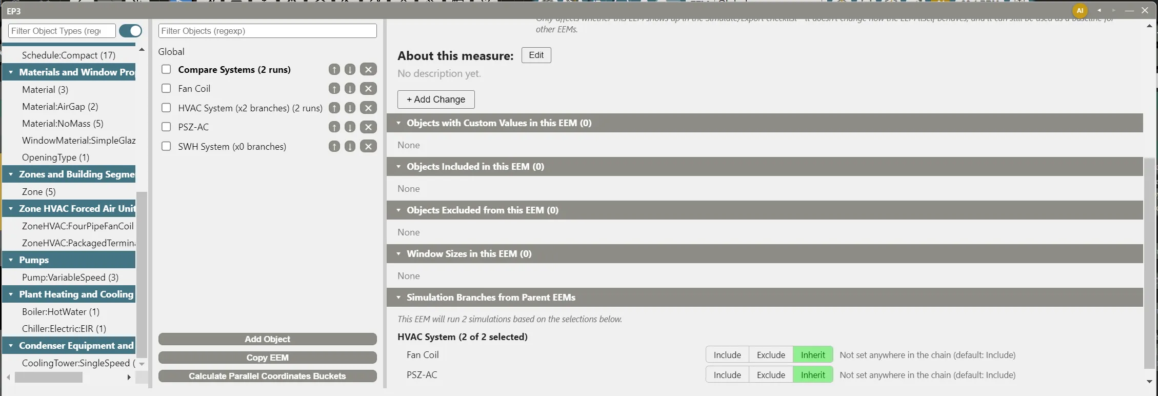
- Run every system from one EEM. Add an EEM built on the built-in HVAC System EEM. It runs once per system, and its Simulation Branches from Parent EEMs section switches systems out (Energy Efficiency Measures (EEMs)).
- Validate and simulate that EEM (§2, steps 9 and 10).
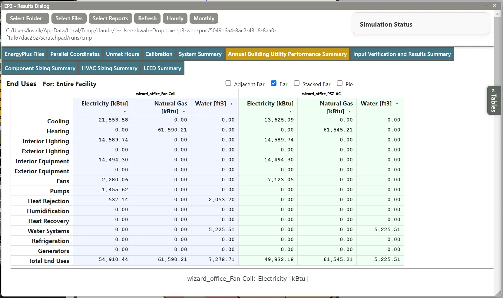
- Compare. In View Results, load the runs with Select Files to read their tables side by side (Viewing and Interpreting Results). Compare energy use only between runs whose Unmet Hours are acceptable: a system that does not meet the loads uses less energy for that reason. The Parallel Coordinates tab plots the systems on one HVAC System axis (Energy Efficiency Measures (EEMs)).
A design that uses different systems for different zones combines the system EEMs in one EEM (Energy Efficiency Measures (EEMs)).
5. An EEM study
- Finish the base model in Global. An EEM should hold only the changes that define it (Energy Efficiency Measures (EEMs)).
- Add one EEM per measure. In Model Settings > Model Alternatives (EEMs), click Add Object, rename the EEM, select it in the EEM dropdown, and make its changes (Energy Efficiency Measures (EEMs)). Its page lists what it changed (§4.4 of that chapter). A measure can also switch objects off or exclude a zone (§4.2, §4.3).
- Sweep a value with a branching EEM. On an EEM with no changes, click Enable Branching, choose the Object Type, the objects, and the Fields, and click + Add Iteration for each value (Energy Efficiency Measures (EEMs)).
- Combine the measures. An EEM built on another (Single EEM) adds to it; an EEM with Multiple EEMs collects the changes of the EEMs it checks (Energy Efficiency Measures (EEMs)). An EEM with a branching EEM in its chain runs once per combination of included iterations, and its row in the EEM list shows the count (§6.3 of that chapter).
- Check the plot before simulating. Calculate Parallel Coordinates Buckets marks the EEMs that can be plotted, and View Parallel Coordinates Plot (Live Preview) draws their inputs (Energy Efficiency Measures (EEMs)).
- Add tariffs for a Total Energy Cost axis (Utility Costs).
- Simulate the combined EEMs (Energy Efficiency Measures (EEMs), Running Simulations).
- Compare on the plot. In View Results, the Parallel Coordinates tab draws one line per run. Select ranges on the axes to find the runs that meet a target, add output axes, and save the chart with Save as HTML… (Energy Efficiency Measures (EEMs)).
6. Calibrating against measured energy use
- Load the measured data. In View Results, open the Calibration tab and click Choose file… for a CSV or Excel file of meter readings or monthly bills. Confirm each column’s fuel and unit and click Save. The mapping is saved with the model, and from then on every simulation also reports the measured fuels’ facility meters hourly (Viewing and Interpreting Results).
- Simulate the EEM that represents the building as operated. A run made before the mapping was saved has no meters to compare; simulate it again.
- Read the comparison. Load the run with Select Files. The tab shows the ASHRAE Guideline 14 NMBE and CV(RMSE), the bias by month, the weather response, and Likely causes.
- Calibrate. Under Calibrate, tick the inputs that may change and set their bounds, choose the Starting EEMs, choose where to Put the result in (a new EEM, named Calibrated by default, or the starting EEM itself), and click Calibrate. EP3 runs a sensitivity simulation per input, fits the inputs within their bounds, applies them, and checks the fit with one more run. Undo reverts the result.
- Check the fitted values for plausibility before building an EEM study (§5) on the calibrated EEM.
7. An ASHRAE 90.1 PRM baseline
- Build the proposed design as in §2 or §3, and save the model.
- Set the PRM inputs: the Climate Zone in General Model Settings (Weather, Climate, and Design Conditions) and the space classifications on each
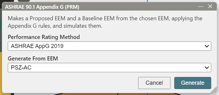
SpaceType’s ASHRAE Space Types tab (Internal Loads, Space Types, and Zone Types). - Generate. Click the balance-scale button (ASHRAE 90.1 performance path) on the toolbar, choose the Performance Rating Method (2019 or 2016) and the EEM in Generate From EEM, and click Generate. EP3 checks the model and the starting EEM’s unmet hours first, then makes a Proposed EEM and a Baseline EEM and simulates them.
- Review the generator’s messages with PRM Messages and the comparison with PRM Report.
ASHRAE 90.1 Performance Rating Method covers each step. For the Energy Cost Budget Method (Section 11 or 12) instead of Appendix G, the same button builds a Proposed and a Budget (§9 of that chapter).
8. Using Atlas along the way
Atlas can help at each stage of these workflows (The EP3 AI Assistant). Its access switch sets what it may do (§3 of that chapter).
- While building: answering questions about EP3 and EnergyPlus from this handbook, creating schedules from a description or an attached file, and proposing small changes to existing objects for you to review and integrate (§6, §8).
- EEM studies: creating EEMs, including branching EEMs, and arranging the parallel coordinates plot (Energy Efficiency Measures (EEMs)).
- After a run: explaining simulation errors and unmet hours, running simulations, and comparing runs (§7, §9).
- Calibration: Suggest with AI fills in the measured data’s mapping, Ask AI which inputs picks the inputs and bounds, and Ask AI to check this fit judges the fitted values. Each fills in the form or reports; nothing changes until you act.
Turn on incognito before the first message to keep real names from a cloud provider (§10).
This handbook is also built into EP3 (Help), where its EnergyPlus links open the EnergyPlus Reference. Technical specifications · Book a demo