Viewing and Interpreting Results
1. Overview
View Results on the top toolbar opens the EP3 - Results Dialog, which reads the files EnergyPlus wrote for each run:
- report tabs: EnergyPlus’s tabular reports, runs side by side, with charts (§3);
- the time-series viewer, with node values drawn on the HVAC diagram (§5);
- Unmet Hours: unmet hours by zone, with the objects behind them and checks of the usual causes (§7);
- Calibration: measured energy use against a run (§8);
- Parallel Coordinates, covered in Energy Efficiency Measures (EEMs);
- Disaggregation: the share of the difference between two EEMs that each change contributes (§9);
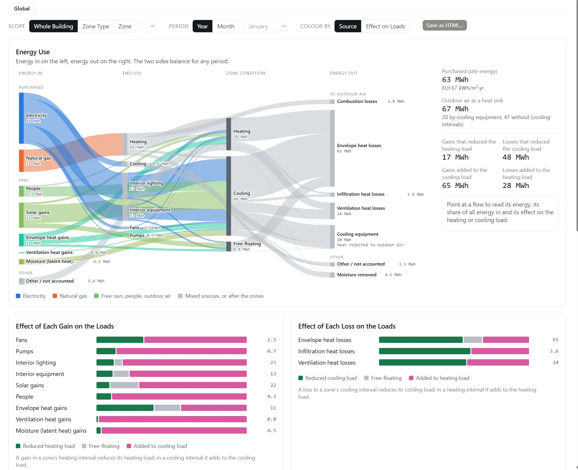
- Energy Flow: a Sankey diagram of the energy bought, the free heat received, and where it went, with the zone condition each gain and loss arrived in (§10);
- EnergyPlus Files: each run’s raw files (§3.5).
View Building Data in the Building Geometry Outliner colors the 3D view by a result and calculates ETTV and RTTV (§6). None of these needs AI. Running simulations is covered in Running Simulations, and error files in Model Troubleshooting and Quality Assurance. The ASHRAE 90.1 PRM generator’s runs are read in its PRM Report (ASHRAE 90.1 Performance Rating Method); for an Energy Cost Budget run, which reports the design energy cost against the energy cost budget, see §9.9 and the unmet load hours in §9.7. Atlas can open the Results dialog at a table, open the time-series viewer with variables picked, and compare runs in the chat (The EP3 AI Assistant).
2. Choosing the runs
2.1 The run folder and Select Files
The dialog opens on the model’s run folder (the folder chosen for this model in this session, else the folder the .ep3 file is saved in) and loads every run in it and its sub-folders: every <name>.epJSON file. An unsaved new model opens empty. The header holds:
- Select Folder…: another folder, such as another model’s runs.
- Select Files: Select Files to View, a checklist of the folder’s runs with Select All and Select None; Save and Update loads the ticked runs. Runs added since the last look start unticked.
- Select Reports: the report tables (§3.1).
- Refresh: reads the runs’ files again after a new simulation.
- A button per time-series frequency the runs reported, such as Hourly (§5).
Each run is named by its path, less the folders all loaded runs share. The header slides away as the page scrolls.
2.2 Simulation Status
The Simulation Status box at the top right lists each run with an icon from its .err file: a green check for no severe errors, a gold check for severe errors, a red cross for a fatal error or no .err file. Point at the box to expand it, and at a run for its error counts; click a run to open its errors (Model Troubleshooting and Quality Assurance). A failed run has no results but still appears here and in the EnergyPlus Files tab.
3. Report tables
Every simulated run requests EnergyPlus’s AllSummary tabular reports, so the report tables need no setup. Each report is a tab; EnergyPlus documents every report and its tables (Output Details and Examples: eplustbl.<ext>).
3.1 Default reports and Select Reports
By default the dialog shows:
| Report | Tables |
|---|---|
| Input Verification and Results Summary | General |
| Annual Building Utility Performance Summary | End Uses |
| Component Sizing Summary | Every table |
| System Summary | Time Setpoint Not Met |
| LEED Summary | EAp2-2. Advisory Messages, EAp2-7. Energy Cost Summary, EAp2-4/5. Performance Rating Method Compliance |
Select Reports opens Select Reports to View, which lists every report the loaded runs contain. Expand a report and tick its tables, then click Update. Reset To Default returns to the set above. Other commonly used tables:
- Annual Building Utility Performance Summary: Site and Source Energy gives the site and source EUI, and Utility Use Per Conditioned Floor Area the use per floor area by fuel (Output Details and Examples: Annual Building Utility Performance Summary).
- HVAC Sizing Summary: zone and system design loads and airflows (Heating and Cooling Loads).
- Equipment Summary and Coil Sizing Details: equipment capacities, efficiencies, and rated conditions.
The table choices, chart choices, and hidden columns are remembered on this computer and apply to every model.
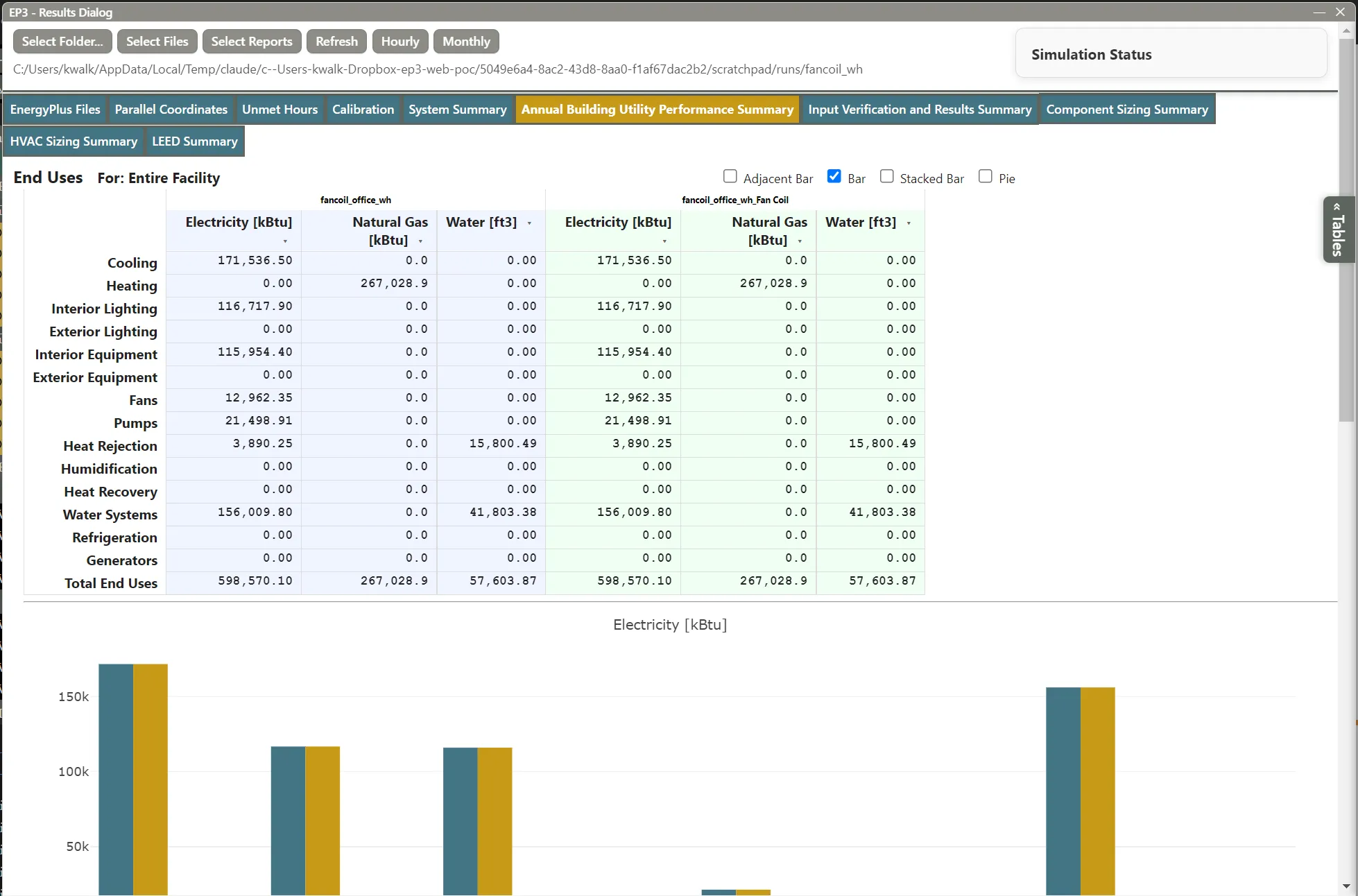
3.2 Reading a table
Each run has its own tinted block of columns, and rows are matched across runs by label; a row a run lacks is blank in its columns. The run name over each block turns from black to red the fewer hours the run simulated, so a design-day-only run stands out.
- The ▾ in a column header hides the column; columns that are all blank or zero start hidden. A hidden column is a thin strip: point at it to highlight the adjacent hidden columns, and click to show them.
- A table EnergyPlus writes per zone or object repeats under a For: heading for each.
- « Tables at the right edge opens an index of the tab’s tables and For: entries, with a filter; click one to jump to it.
- Each column’s numbers share one number of decimals, so the decimal points line up, chosen from the column’s largest value. Hours keep what EnergyPlus counted: setpoint-not-met hours come in quarter-hour steps, so a column with 4,263.5 hours not comfortable also shows 51.5 and 0.5 hours not met, never 52 and 1.
- Pointing at a number shows ⊕, which adds it as a parallel coordinates output axis (Energy Efficiency Measures (EEMs)).
3.3 Units
Tables follow the SI / IP setting. EP3 asks EnergyPlus for tabular energy in kWh when the model has no table style, and reads whatever units a run wrote, from any EnergyPlus version and any table style (EnergyPlus Versions). A unit EP3 does not convert is shown as EnergyPlus wrote it, and the message line names it. In IP energy shows in kBtu, and other units convert to their IP equivalents, rounded to two decimals. A site EUI of 100 kWh/m² shows as 100 × 3.412 kBtu/kWh ÷ 10.764 ft²/m² = 31.70 kBtu/ft².
3.4 Charts
Each table’s header row has four chart boxes:
- Bar: a chart per column per run, with a bar for each row.
- Adjacent Bar: a chart per column, with the runs’ bars side by side for each row.
- Stacked Bar: a chart per column, with a bar per run made of the rows stacked.
- Pie: a pie per column per run.
Charts leave out total rows, blank rows, hidden columns, and columns that are zero in every run. End Uses shows a bar chart until changed. A chart’s toolbar, shown on hover, has a camera button that saves it as a PNG.
3.5 The EnergyPlus Files tab
The dialog opens on EnergyPlus Files, which lists each run with a button per file it has: Errors (.err), IDF (the run’s .epJSON), Tables (EnergyPlus’s HTML report), RDD (every variable the run could report), Output Variables (.csv), and ESO (.eso). Each opens in the computer’s application for that file type. The report tables are also in the run folder as CSV (<run>tbl.csv).
4. What a run reports over time
Time-series output exists only for the variables the export requested. Every export requests:
- the site outdoor dry-bulb, wet-bulb, and dew-point temperatures, and each zone’s Zone Mean Air Temperature, at the model’s Default Reporting Frequency for Output:Variable (The EP3 Interface and Model Settings);
- each zone’s mean air temperature, thermostat heating and cooling setpoints, occupant count, and delivered sensible heating and cooling rates, and each air loop’s Air System Simulation Cycle On Off Status, at Timestep when the model reports by timestep and otherwise Hourly;
- each zone’s occupied unmet heating and cooling time, monthly;
- the temperature, mass flow rate, and setpoint at every node a setpoint manager sets (Air Loops, Branches, and Nodes).
The second and third groups feed the Unmet Hours tab (§7). Request other variables before simulating:
- on an object’s Outputs tab, which has a sub-tab for the object and for each object it contains, listing the variables that object type reports, each with Report? and an optional EMS Sensor Name, plus a Reporting Frequency and Schedule (Heating and Cooling Loads). The dialog’s epJSON button shows the
Output:Variableobjects the export will write for the open sub-tab; - in the View Building Data picker, for surface, window, zone, and space variables (§6.1);
- with a
NodeReport, for chosen HVAC nodes (Air Loops, Branches, and Nodes); - with an
Output:Variableobject in the main object dialog, for any variable name from the Input Output Reference or a run’s RDD file.
5. The time-series viewer
5.1 Opening and charting
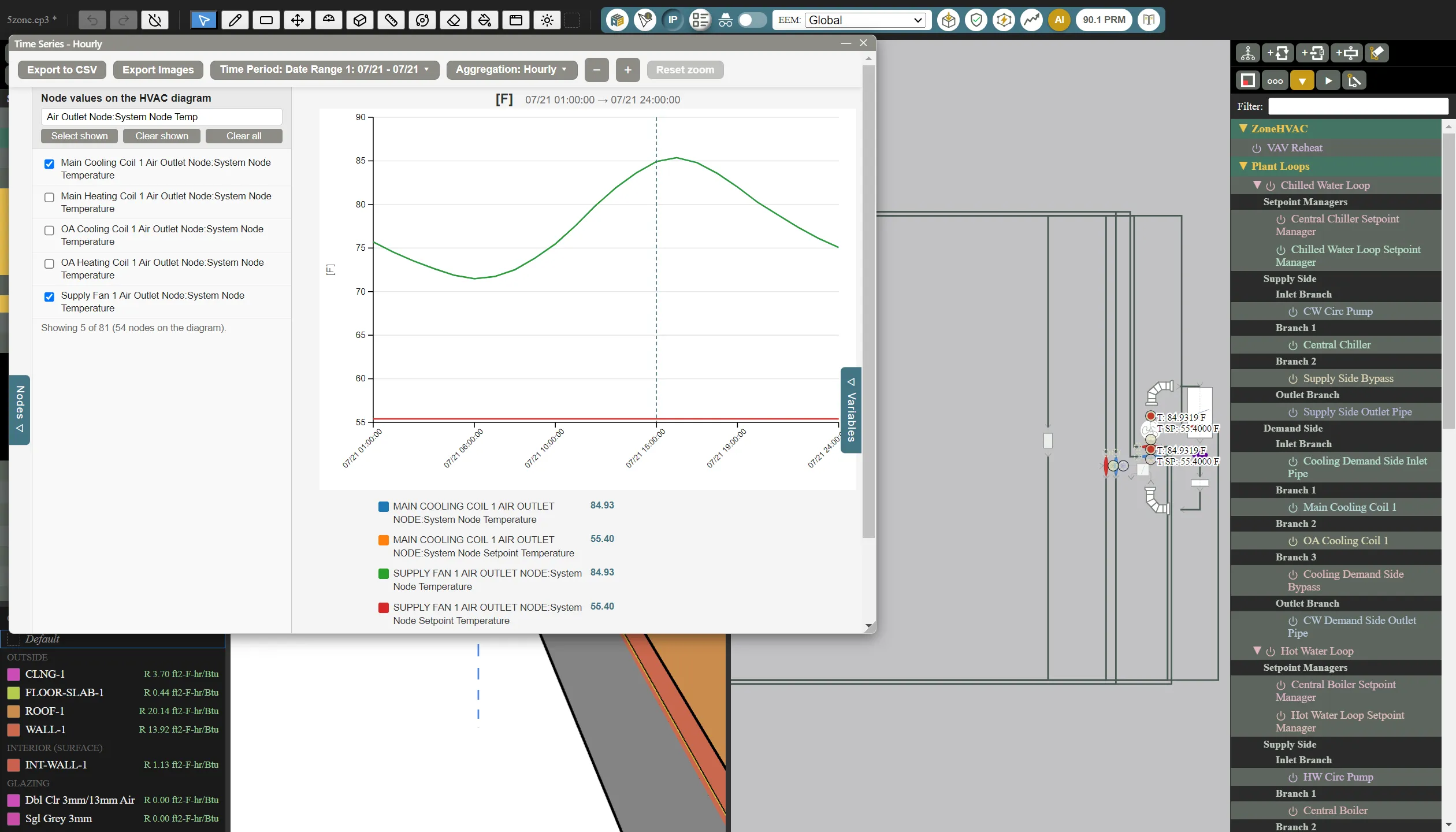
A frequency button in the Results dialog’s header, such as Hourly, opens Time Series - Hourly for every loaded run that reported at that frequency. The Variables ▷ panel lists each run’s variables under a collapsible heading; the filter narrows the list (up to 300 are listed at a time), with Select shown, Clear shown, and Clear all. Tick a variable to chart it.
Each unit gets its own chart. Drag across a span to zoom to it; a span over more than one day widens to whole days, so dragging across a week shows that week from its first hour to its last; + and − zoom about the center, and Reset zoom or a double-click shows the whole period. The legend shows each line’s value at the pointer; click an entry to hide or show its line. Values follow the SI / IP setting. Heating and Cooling Loads works an example with zone loads.
5.2 Time Period and Aggregation
Click Time Period or Aggregation to open its menu. Time Period lists the file’s date ranges (Date Range 1, Date Range 2, and so on): EnergyPlus writes the sizing periods and the run period one after another, and EP3 starts a range wherever the dates jump. With several runs loaded, the ranges come from the first run, and the others are matched to it by date and time.
Aggregation rolls the data up to Daily, Monthly, or Annual. Value Type (all variables) is EnergyPlus default (Sum or Average), as EnergyPlus tags each variable (energies summed, rates and temperatures averaged), or Sum, Average, Minimum, or Maximum. A ticked variable’s menu overrides it for that variable.
5.3 Aliases and calculated variables
A ticked variable gets a tag (v1, v2, … in the order ticked) and an alias field; the alias replaces its name in the legend and can be used in formulas.
+ Add calculated variable adds a row with a Name, a Formula, and Units. A formula combines aliases or tags with + - * / ^ ( ), abs, sqrt, min, and max, such as v1 - v2. Formulas are evaluated in SI and not converted, so give SI units. A calculated variable rolls up by Sum unless the Value Type says otherwise. Its box turns it off; Remove deletes it.
5.4 Exporting
Export to CSV saves the charted values as shown (time period, aggregation, and units), a column per variable, prefixed by run when several are loaded. Export Images saves each chart as a PNG in a chosen folder.
5.5 Node values on the HVAC diagram
When one run is loaded and it reported system node variables, the Nodes ▷ drawer on the left lists each diagram node with its reported variables. Tick variables to label their nodes on the HVAC diagram with the value at the chart pointer’s time. The drawer has a filter and Select shown, Clear shown, and Clear all. Nodes of a replicated loop’s copies are not labeled, and node viewing is off with several runs loaded.
6. Results on the 3D model
6.1 Coloring by a variable
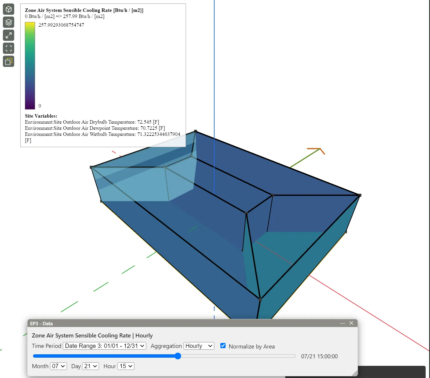
View Building Data in the Building Geometry Outliner opens EP3 View Geometry Data, listing every surface, window, zone, and space variable. Expand a variable for its frequencies: a frequency with results in the active EEM’s latest run is a button that colors the model, and the box beside each frequency requests the variable for every object of its type in the next run. Variables with results are bold; only with results hides the rest, and Refresh reads the run again. RESULTS MAY NOT BE CURRENT means the model has changed since the run.
A frequency button opens EP3 - Data: Time Period, Aggregation, Value type (when aggregating), Normalize by Area (where it applies), a time slider, and month, day, and hour menus. Faces are colored by their value at that time, on a scale from the period’s lowest value to its highest; a zone’s or space’s value colors all its faces, and faces with no data are grey. Point at a face for its value; the legend shows the range and the site variables’ values. Close EP3 - Data, or click View Building Data again, to turn the coloring off. Set the EEM menu to the EEM whose run you want. Heating and Cooling Loads works an example.
6.2 ETTV and RTTV
The picker’s ETTV and RTTV data row calculates Singapore’s envelope (wall) and roof thermal transfer values from the active EEM’s latest run, following BCA’s Guidelines on ETTV: the run’s U-factors, areas, and SHGCs from the Envelope Summary, the guidelines’ solar data and correction factors, and the shade cast on each window by its surroundings, inset, overhang, and fins. The weather file is not used.
ETTV = 12(1 − WWR)Uw + 3.4(WWR)Uf + 211(WWR)(CF)(SC)
RTTV = 12.5(1 − SKR)Ur + 4.8(SKR)Us + 485(SKR)(CF)(SC)
where WWR is the window-to-wall ratio, SKR the skylight-to-roof ratio, Uw, Uf, Ur, and Us the U-factors (W/m²·K) of the opaque wall, the windows, the opaque roof, and the skylights, CF the guidelines’ correction factor for the surface’s orientation and tilt, and SC the shading coefficient of the glass and its external shading together. EP3 takes the glass’s SC as SHGC ÷ 0.87.
For example, a wall with WWR 0.4, Uw 0.5 W/m²·K, Uf 2.0 W/m²·K, CF 0.9, and SC 0.5:
ETTV = 12(0.6)(0.5) + 3.4(0.4)(2.0) + 211(0.4)(0.9)(0.5) = 3.60 + 2.72 + 37.98 = 44.30 W/m² (14.04 Btu/h·ft²)
The solar term dominates, so shading and a lower SHGC lower ETTV most.
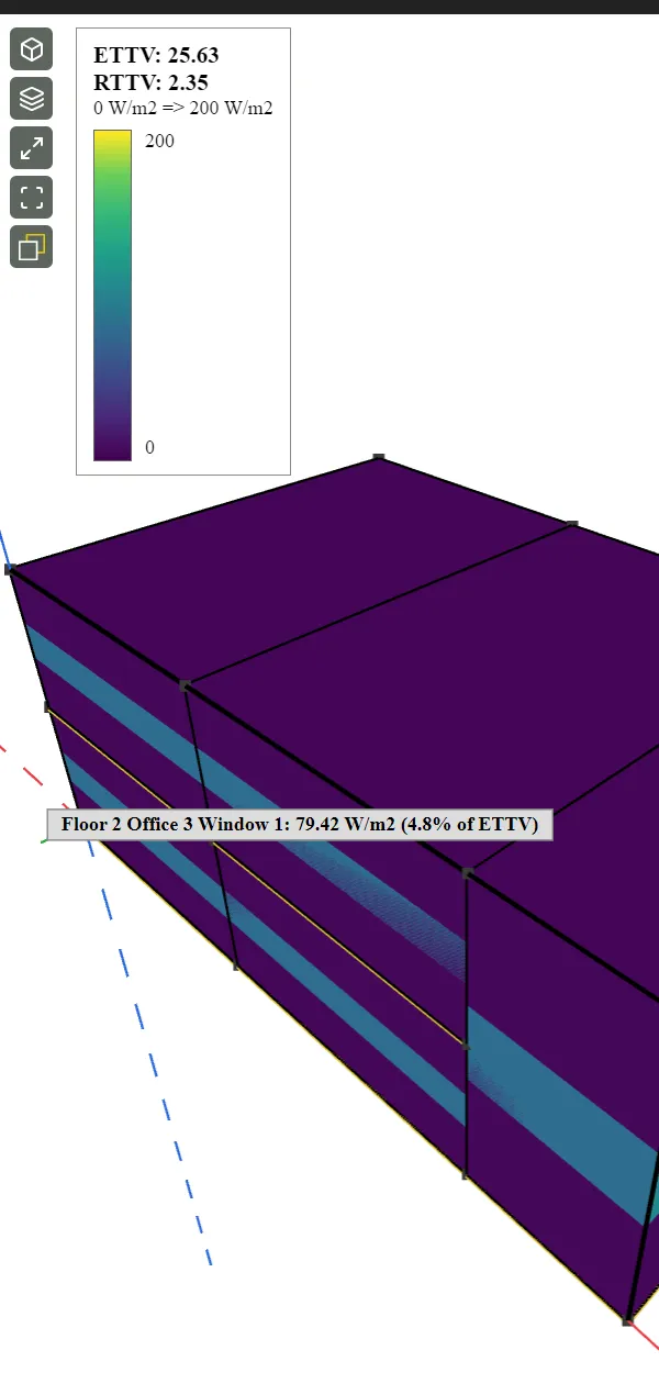
Calculate (then Recalculate) shows ETTV and RTTV in W/m², with any warnings, such as a surface with no U-factor in the report. View colors each wall, roof, and window by its contribution per unit area on a fixed 0 to 200 W/m² scale; point at a face for its share. The result is kept per EEM for the session and marked when the model changes. The totals are added to the run’s results as the ETTV and RTTV Calculations report, which Select Reports can show.
7. The Unmet Hours tab
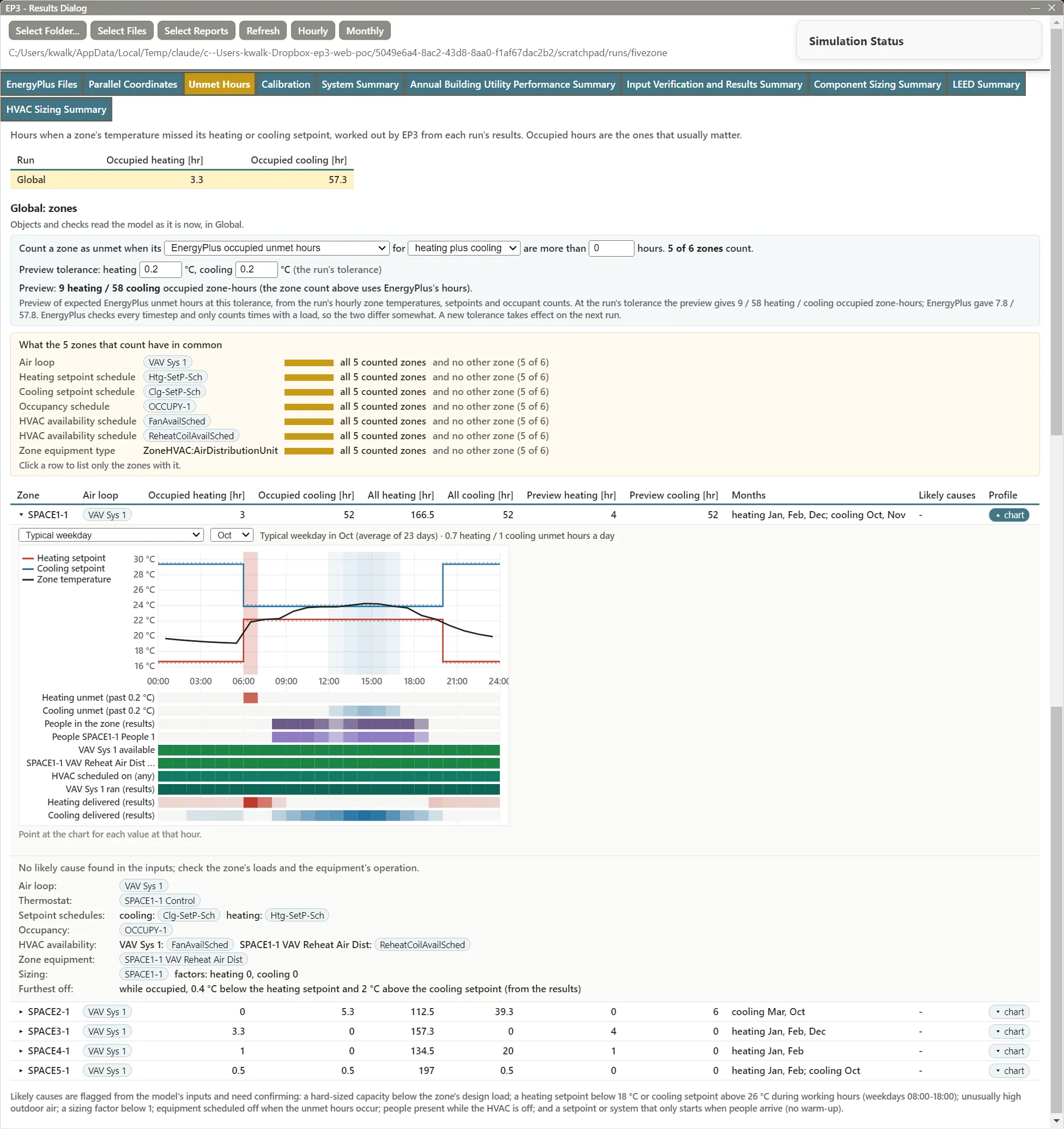
The Unmet Hours tab finds the zones whose temperature missed the heating or cooling setpoint, shows what controls them, and flags likely causes. Atlas starts from the same analysis when asked about unmet hours (The EP3 AI Assistant); fixing the causes is covered in Model Troubleshooting and Quality Assurance. Temperatures and tolerances in this tab follow the model’s unit system.
7.1 Runs and zones
The first table lists each run’s occupied heating and cooling unmet hours (Annual Building Utility Performance Summary, Comfort and Setpoint Not Met Summary). Click a run to show its zones; the worst run is shown first.
The zones table (System Summary, Time Setpoint Not Met) lists the zones that count (§7.2), worst first, with the Air loop serving each (traced from its terminals and inlet nodes through zone splitters and supply plenums), occupied and all-hours heating and cooling unmet hours, the preview’s hours when the run has them, the Months the occupied hours fall in, Likely causes tags (§7.3; point at one for its text), and the Profile chart (§7.4).
Click a zone to expand it: the checks with their objects, then Air loop, Thermostat, Setpoint schedules, Occupancy, HVAC availability, Zone equipment, Sizing, and, with the preview, Furthest off (the largest occupied shortfall below the heating setpoint and excess above the cooling setpoint). Each object is a link that selects and opens it. Objects and checks read the model as it is now, in the EEM the run simulated.
7.2 Criteria and the tolerance preview
The criteria bar reads: Count a zone as unmet when its [measure] for [heating plus cooling, heating, or cooling] are more than [N] hours. The measures are:
- EnergyPlus occupied unmet hours (the default) and EnergyPlus unmet hours (all hours);
- EP3 preview: occupied hours past a tolerance and EP3 preview: all hours past a tolerance.
EnergyPlus counts time as unmet when the zone is more than a tolerance below its heating setpoint or above its cooling setpoint. The tolerance is set by OutputControl:ReportingTolerances: 0.2 °C (0.36 °F) for each when the model has none.
The Preview tolerance fields recount the run’s hours at another tolerance from its zone temperatures, setpoints, and occupant counts, without simulating. Editing a tolerance switches to the matching preview measure, so the zone count, commonalities, and zones table follow it. The totals show under the fields, with the preview and EnergyPlus counts at the run’s tolerance for comparison. The two count different things, and a line under the totals says how. The preview adds up each zone’s hours, so two zones unmet in the same hour count twice; the runs table gives EnergyPlus’s building hours, where that hour counts once. EnergyPlus also checks every timestep while a zone has a load, while the preview works from the zone temperatures the run reports. From hourly results, a zone that falls short for only part of an hour (often at start-up) may not count in the preview, so its totals can be well below EnergyPlus’s. For example, one Wizard office run gave 51.5 occupied heating hours in EnergyPlus and about two thirds as many zone-hours in the preview at the same tolerance. reset to the run’s tolerance returns to it. Use this tolerance in the model… writes it to OutputControl:ReportingTolerances in Global or the run’s EEM (creating the object in Global if there is none), for the next run.
Runs simulated before EP3 requested the zone operation variables have no preview and no chart temperatures; simulate again.
7.3 Likely causes
Each check looks for one common cause in the zone’s inputs and names the objects involved, quoting setpoints, capacities, and outdoor air rates in the model’s unit system. A check is a lead to confirm, not a finding:
| Tag | Flags |
|---|---|
| Capacity | A hard-sized capacity on the zone’s equipment, coils, or fans below the zone’s design load from the HVAC Sizing Summary (or any hard-sized capacity, without that table) |
| Setpoint | A heating setpoint below 18 °C (64.4 °F) or a cooling setpoint above 26 °C (78.8 °F) for more than 10% of working hours (weekdays 08:00 to 18:00) |
| Outdoor air | An outdoor air specification above 0.003 m³/s·m² (0.59 cfm/ft²), 0.03 m³/s per person (63.6 cfm per person), or 6 air changes per hour |
| Sizing factor | A heating or cooling sizing factor above 0 and below 1, in Sizing:Zone or Sizing:Parameters |
| Availability | Equipment, coils, or fans scheduled off all year, or for whole months, including the months the hours happen |
| Occupied, HVAC off | People in the zone while every air loop and unit serving it is scheduled off, for at least 10 hours and 1% of occupied hours |
| No warm-up | On more than half the occupied days, the heating or cooling setpoint, or the system, first comes on in the hour people arrive |
The setpoint and schedule checks evaluate Schedule:Compact and Schedule:Constant hour by hour; other schedule types are listed as not evaluated.
7.4 Commonalities and the zone profile chart
What the N zones that count have in common lists the air loop, thermostat, setpoint schedules, occupancy schedule, HVAC availability schedules, and zone equipment types shared by at least half of those zones, with how many other zones share them (“and no other zone”). Click a row to list only the zones with it; show all clears the filter.
Point at a zone’s ▾ chart button to preview its day profile; click to pin it under the row. It shows a Typical weekday, Typical Saturday, or Typical Sunday of a month (the zone’s worst at first), or the preview’s Worst day: the setpoints with the tolerance dashed, the zone temperature with the hours past the tolerance shaded, and strips for Heating unmet and Cooling unmet (the share of days unmet at each hour), the people in the zone, each occupancy and availability schedule, HVAC scheduled on (any), when each air loop ran, and the heating and cooling delivered. Point at the chart for each hour’s values. A zone unmet in the hour people arrive, with its system starting that hour, points to warm-up; one unmet all afternoon while the cooling delivered stays at its peak points to capacity.
7.5 Why the hours happen
Why the hours happen, above the air loop section, sorts the run’s unmet zone-hours by cause, from the zones’ hourly unmet time, setpoint schedules, and system availability:
- Warm-up — the first unmet hours after the setpoint or the system switches to occupied (within 3 hours of the start, 5 after a weekend or holiday), when the zone then held its setpoint. It shows what the warm-up starts with: the thermostat, the system schedule, or both. Starting the setpoint and the fans earlier, or a smaller setback, shortens it.
- Capacity — every other unmet hour, with the share that falls in the coldest or hottest tenth of the year’s hours. Larger equipment or a lower load addresses these.
- Control — people are present while the system is scheduled off or the setpoint is at its setback value. The schedules disagree; fix them in the model.
A summary line gives the hours with any zone unmet and the zone-hours by cause. The table can be grouped by zone, by setpoint schedule (a schedule’s fix covers every zone that shares it), or by air loop. A run made before this version has only monthly unmet hours, and the section says so. The ASHRAE 90.1 PRM generator uses the same sort to choose its warm-up fixes (ASHRAE 90.1 Performance Rating Method), as does the Energy Cost Budget Method (§9.7).
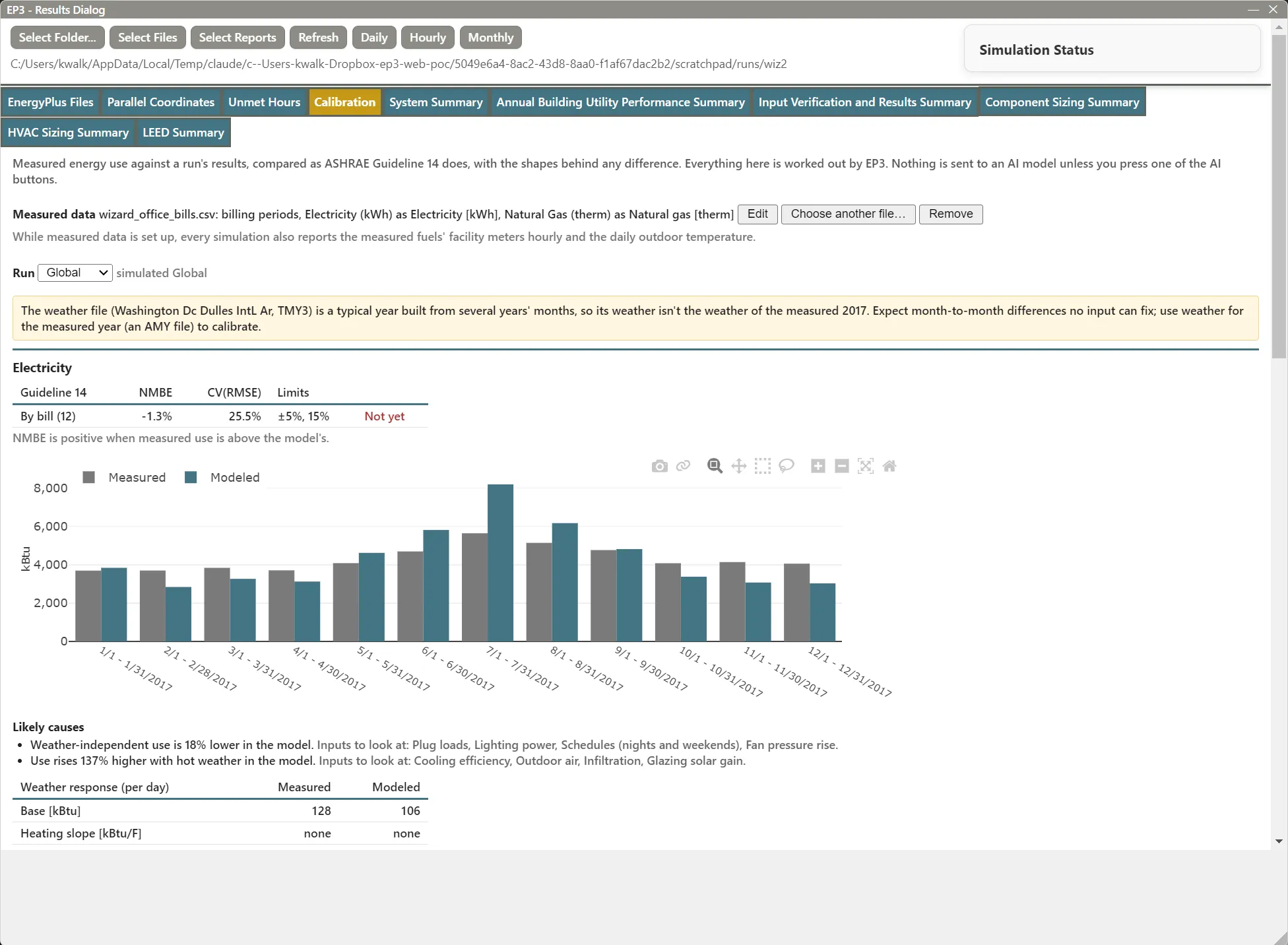
8. The Calibration tab
The Calibration tab compares a run with measured energy use, following ASHRAE Guideline 14, and can adjust the model to fit the measurements.
8.1 Setting up measured data
Choose file… takes a CSV or Excel file of meter readings (15-minute to daily) or bills. EP3 detects the layout and fills in How to read file: Sheet (Excel), Interval, Date (or Period start and Period end for bills), Dates are written (month/day/year or day/month/year, with a warning when every date reads either way), and Each time marks (the start or end of its interval). For each numeric column, set Measures (a fuel for the whole building, or (not used)) and Unit (kWh, MWh, Wh, kW average demand, therm, ccf, MMBtu, kBtu, GJ, MJ, or m³). For ccf and m³, enter the bill’s heat content in kWh per unit; EP3 starts at 30.39 kWh per ccf (1.037 therm) and 10.55 kWh per m³ (38 MJ/m³).
A line under the columns shows how many readings the settings read, over what dates. Save stores the mapping with the model; the file is read from where it is each time the tab opens. Edit, Choose another file…, and Remove change it later. Suggest with AI fills in the form from the headers and first five rows for you to check.
While measured data is set up, every export requests each mapped fuel’s facility meter (such as Electricity:Facility) hourly and the outdoor dry-bulb daily, so simulate again after setting it up.
8.2 Reading the comparison
Choose the Run. Warnings come first: a typical-year weather file, which leaves month-to-month differences no input can fix (use weather for the measured year); a weather file for another year; and missing meters. Each fuel then has:
- Guideline 14: NMBE and CV(RMSE) by month (or bill), and by hour for interval data, against the limits (±5% and 15% monthly, ±10% and 30% hourly), marked Calibrated or Not yet. NMBE is positive when measured use is above the model’s.
- A bar chart of measured and modeled use per month or bill.
- Likely causes, with the inputs to look at; a high base load, for example, points to plug loads, night lighting, or schedules.
- Weather response (per day): a change-point fit of daily energy against outdoor temperature, measured and modeled (Base, Heating slope, Heating below, Cooling slope, Cooling above, R²), plus Weekday night base, Weekday peak, Operating hours, and Weekend / weekday for interval data.
- For readings more frequent than daily, By hour and day of week: modeled, measured, and ratio grids over the year, a season, or a month. The ratio is blue where the model is low and red where it is high.
Energy shows in kWh (SI) or kBtu (IP). With n periods, measured values M, and modeled values S:
NMBE = 100 × Σ(M − S) ÷ ((n − 1) × mean M)
CV(RMSE) = 100 × √(Σ(M − S)² ÷ (n − 1)) ÷ mean M
For example, 12 monthly bills averaging 10,000 kWh, with the measured total 4,400 kWh above the model and squared differences summing to 15,840,000 kWh²:
NMBE = 100 × 4,400 ÷ (11 × 10,000) = 4.0%
CV(RMSE) = 100 × √(15,840,000 ÷ 11) ÷ 10,000 = 100 × 1,200 ÷ 10,000 = 12.0%
Both are within the monthly limits, so the fuel is Calibrated. In IP the same bills average 34,121 kBtu with a 15,013 kBtu difference, and the percentages are unchanged.
8.3 Calibrating
The Calibrate section adjusts inputs by multipliers to fit the measured months or bills. Tick the inputs that may change and set each one’s range in From and To (percent); the inputs the likely causes point to start ticked.
| Input | Changes | Default range |
|---|---|---|
| Lighting power | Lights |
−30% to +30% |
| Plug and process loads | ElectricEquipment and GasEquipment |
−50% to +50% |
| Infiltration | ZoneInfiltration:DesignFlowRate |
−50% to +100% |
| Outdoor air | DesignSpecification:OutdoorAir |
−50% to +50% |
| Cooling efficiency (COP) | DX coils, chillers, VRF | −30% to +30% |
| Heating efficiency | Furnaces, boilers, heat pumps (fractions capped at 1) | −20% to +20% |
| Fan pressure rise | Fan:ConstantVolume, Fan:VariableVolume, Fan:OnOff, Fan:SystemModel |
−30% to +30% |
| Hot water use | WaterUse:Equipment |
−50% to +50% |
A multiplier applies to every object of its classes, including per-Space and per-Zone values. Choose one or more Starting EEMs (two HVAC systems, say, to compare their fits) and Put the result in a new EEM building on each (named Calibrated by default) or the starting EEM itself.
Calibrate runs, for each starting EEM, one simulation as it is, one per input at its upper bound, and one to confirm: three inputs on one starting EEM take 1 × (3 + 2) = 5 simulations. EP3 finds the multipliers within the ranges that best match every fuel’s months or bills, weighting each fuel by its mean so a small gas bill counts as much as a large electricity bill, applies them, and runs the result. The outcome lists each multiplier, marked (at its bound) or (no effect), and each fuel’s NMBE and CV(RMSE) before and after. The temporary sensitivity EEMs are removed and their run files kept; Undo reverts the result.
The fit cannot tell a plausible cause from an implausible one: a multiplier at its bound, or one that fixes one fuel by worsening another, means looking for another cause. Ask AI which inputs and Ask AI to check this fit send EP3’s summary (never the readings) to Atlas, which ticks inputs or rates each multiplier for you to review. They need Atlas access of Analysis or above; Suggest with AI needs Help (The EP3 AI Assistant).
9. The Disaggregation tab
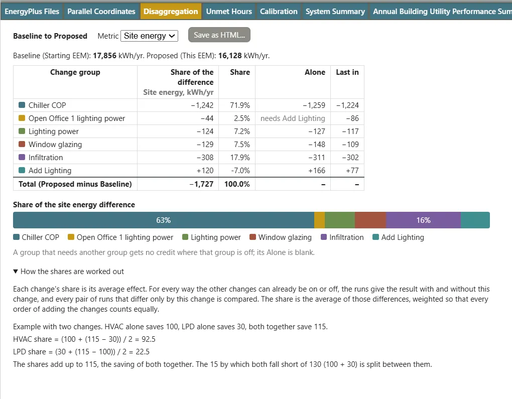
The Disaggregation tab shows what each change group contributes to the difference between two EEMs. It appears when a loaded run came from a disaggregation (Energy Efficiency Measures (EEMs)), and it reads the runs the dialog has already loaded. View Results on the EEM’s Disaggregation tab opens the dialog on it.
9.1 The table and the bar
The tab names the comparison, then gives a Metric menu: Site energy, Utility cost, or Site EUI. Site energy and EUI follow the SI / IP setting (kWh and kWh/m², or kBtu and kBtu/ft²), and cost is as the tariff reports it. A line under the menu gives the two end values, such as Baseline (Starting EEM): 17,856 kWh/yr. Proposed (This EEM): 16,128 kWh/yr.
The table has a row for each change group and a Total row, the This EEM value minus the Starting EEM value. A decrease is negative. The columns are:
- Share of the difference: the group’s share of the total in the metric’s unit. The shares add up to the total.
- Share: the same as a percentage of the total. A group that works against the total has a negative percentage, such as the added lighting in the example, or the savings in a cost comparison where the total is an increase. The percentages can add up to more than 100% on either side of the total.
- Alone: the group’s effect on its own, the run with only that group on minus the Starting EEM run. A group that depends on another group shows needs
<group>, since it has no effect alone. - Last in: the effect of adding the group to a model that already has every other group, the This EEM run minus the run with every group but this one.
Under the table, a bar shows the shares with the same signs: groups that lower the metric sit left of a zero line, groups that raise it right of it, each segment as wide as the size of its share and in its group’s color from the legend. Segments large enough to hold it carry the table’s percentage, so a group that raises the cost can read 137.9% while the savings read negative. A line under the bar says how to read it.
Save as HTML… writes the table, bar, notes, and explanation to one self-contained page that opens in any browser.
When the loaded runs belong to more than one disaggregation, a menu picks the one to show, named by its comparison. When This EEM makes several runs, a second menu picks the run, named by its iterations.
9.2 How the shares are worked out
Disaggregation separates changes that interact. Two changes together rarely give the sum of what each gives alone: reduced lighting power also reduces cooling, so the lighting saves less energy when the HVAC is already efficient. The share of a change is its average effect over every way the other changes can already be on or off. For every such state, the runs give the result with and without the change, and the share is the average of those differences, weighted so that every order of adding the changes counts equally. Each interaction is divided between the changes that cause it, and the shares always add up to the total.
An example with two changes. HVAC alone saves 100, lighting power density (LPD) alone saves 30, and both together save 115, 15 less than 100 + 30:
- Added first, HVAC saves 100. Added after LPD, it saves 115 − 30 = 85. HVAC share = (100 + 85) / 2 = 92.5.
- Added first, LPD saves 30. Added after HVAC, it saves 115 − 100 = 15. LPD share = (30 + 15) / 2 = 22.5.
The shares add up to 115, and the 15 by which the two changes fall short of 130 is divided between them. The same text is in a collapsed How the shares are worked out under the bar.
9.3 When figures are missing
A figure is worked out only from the runs that are loaded:
- Share needs every combination, so run Every combination (§9.4). With fewer runs the column shows – and a note reads
Some combinations were not run, so shares can't be worked out; run Every combination. - Alone needs the runs with a single group on, and Last in needs the runs with all but one group on. Both come with One at a time and All but one.
- The Total needs the Starting EEM and This EEM runs. A note names a missing one, and without the This EEM run no figure is given.
- A loaded run with no value for the metric, such as a failed run or a model with no tariff for Utility cost, is left out, and a note says how many.
- A combination that the Disaggregation tab marked not run has no run of its own. Where it repeats another run’s model, that run’s value is used; where a dependent group is on without the group it needs, the value of the same combination with the dependent group off is used, so that group gets no credit there. The shares still add up.
Shares are worked out for up to 12 change groups. Above that the tab says there are too many groups.
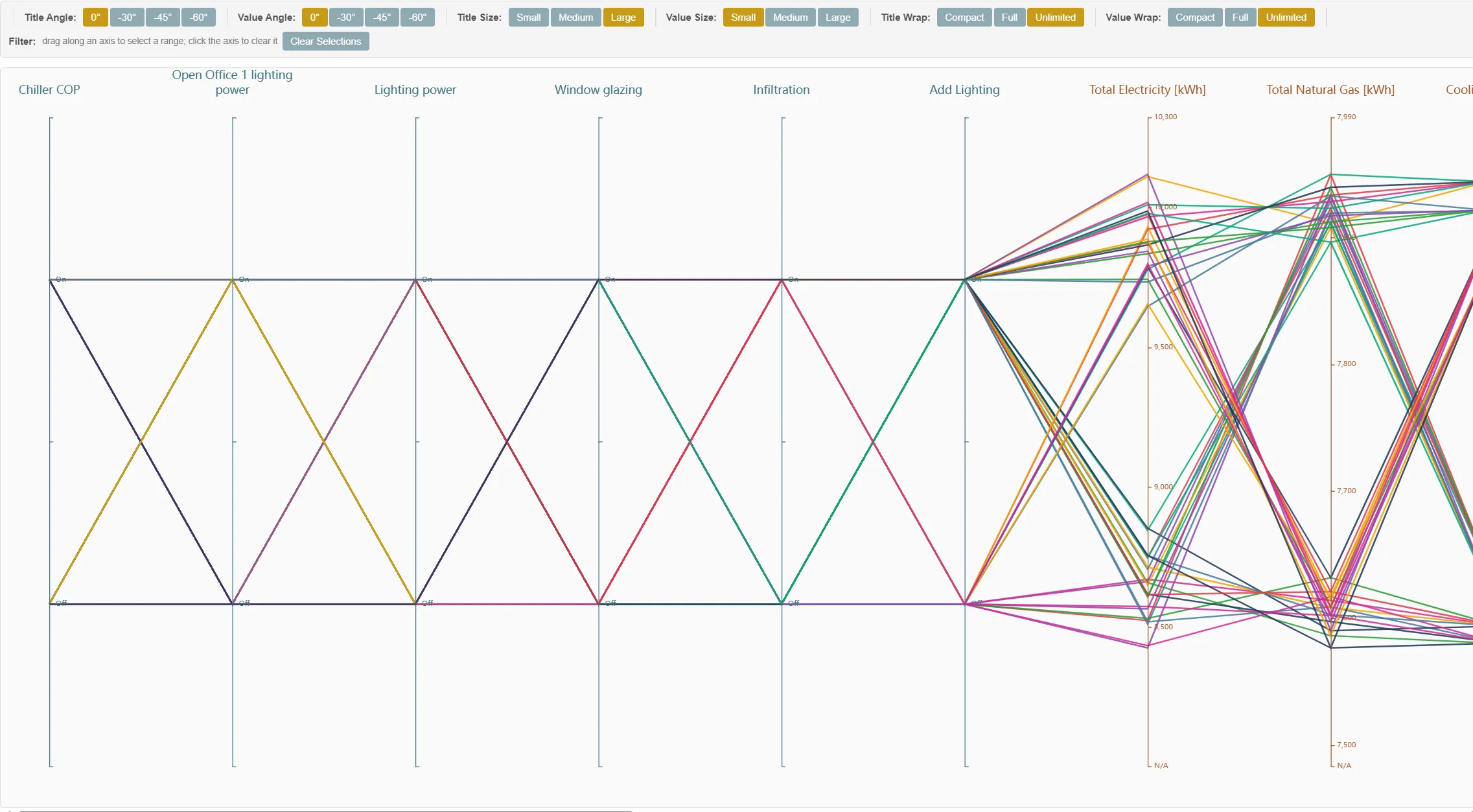
9.4 The runs in Parallel Coordinates
The runs of a disaggregation also appear in the Parallel Coordinates tab, with one input axis for each change group (Energy Efficiency Measures (EEMs)). A run reads On or Off on an axis, or the iteration’s name for a group with levels. Runs of other EEMs read N/A. When two disaggregations are loaded, the axes read <comparison>: <group>. The plot relates each combination of changes to the outputs, with the output axes for energy, cost, and unmet hours.
10. The Energy Flow tab
The Energy Flow tab draws a run’s energy as a Sankey diagram: the energy bought and the free heat received, the end uses, the condition each zone was in when each gain and loss arrived (heating, cooling, or free-floating), and where the energy left. Energy in equals energy out for any period, so each flow can be followed from its source to its destination. Free heat from the sun, people, and the outdoor air that heat pumps draw on appears beside the energy bought, so the diagram shows the whole balance.
The zone condition shows whether each gain and loss helped. A gain that arrives while a zone is heating reduces the heating load; the same gain arriving while the zone is cooling adds to the cooling load.
10.1 Runs and Not Available
The tab has a sub-tab for each loaded run and reads a run’s files only while its sub-tab is selected. It needs the zone results at the run’s hourly or timestep frequency and the run’s monthly end use tables. A run without them shows Not Available with the reason. The usual reasons are a run made before the tab existed, a run made with Energy Flow outputs turned off (§10.7), and a model with no zones. For the first two, turn the setting on and simulate again.
10.2 Controls
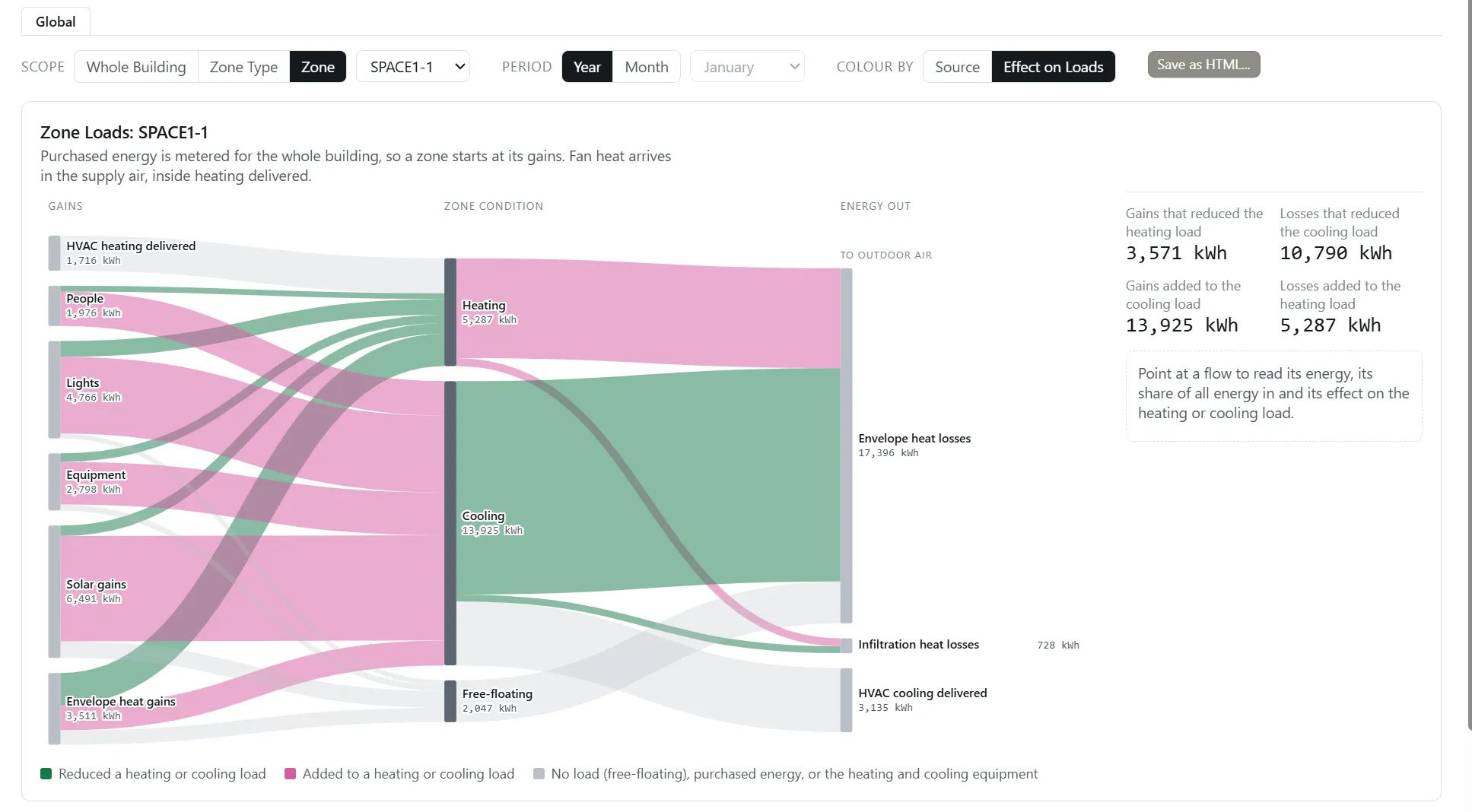
- Scope: Whole Building, Zone Type, or Zone, with a menu to pick the Zone Type or zone. Purchased energy is metered for the whole building, so a Zone or Zone Type view starts at the zone’s gains and has no end uses. Fan heat arrives in the supply air and is included in the heating or cooling delivered. A Zone Type view adds up its zones. Zones that no Zone Type holds, or that cannot be matched to the current model, are grouped under Other zones, with a note.
- Period: Year, or Month with a menu of the months the run simulated.
- Colour by: Source or Effect on Loads.
- Save as HTML…: writes the diagram, the bars, the tables, and the notes to one self-contained page that opens in any browser.
Source colors each flow by where it came from. Electricity is blue and natural gas orange. Every other source takes a color from its name, within a family for its category: purchased fuels and district energy in amber to olive, free heat in greens, air from other zones in violet, and the lights and equipment of a zone view in cyan. A source keeps its color in every scope, period, and run. Flows that mix sources, and flows after the zones, are grey. Effect on Loads colors each flow by its effect on the zones’ heating and cooling loads: green where it reduced a load, magenta where it added to one, and grey in a free-floating zone, for purchased energy, and for the heating and cooling equipment.
10.3 Reading the diagram
A Whole Building diagram is titled Energy Use and has four columns:
- Energy In: Purchased energy (electricity, natural gas, other fuels, district heating and cooling), and Free energy: solar gains, people, heat gains through the envelope, infiltration, and ventilation, moisture (latent heat) gains, on-site generation, and the source a heat pump draws on (outdoor air, a water loop, or the ground). Under Other, Chiller false load is the heat EnergyPlus rejects beyond the cooling delivered.
- End Use: EnergyPlus’s end uses, such as Heating, Cooling, Interior lighting, Fans, and Pumps, each fed by the fuels that supply it.
- Zone Condition: Heating, Cooling, and Free-floating. Every gain and loss takes the condition its zone was in for that interval (an hour, or a timestep), and the zones are added up.
- Energy Out: the To outdoor air group holds the envelope, infiltration, and ventilation heat losses, the Economizer’s free cooling, the heat the Cooling equipment rejects, Combustion losses, Heat pump defrost and crankcase electricity, and exterior lighting and equipment (Outdoors). Combustion losses is the fuel burned beyond the heat delivered by boilers, fuel-fired heating coils (furnaces, unit heaters, and the gas coils of other equipment), fuel-fired water heaters, and direct-fired chiller-heaters, with their parasitic energy; it leaves in the flue gas. Moisture removed, hot water Down the drain, Water heater standby losses, and Equipment lost heat (equipment energy that never reaches the zone) appear when the model has them. Other / not accounted is the energy the meters hold that the zones do not explain, or the reverse (§10.5).
Outdoor air is both a source and a sink. A heat pump in heating draws heat from it (Outdoor air under Free), and the cooling equipment and the losses of cooling zones put heat into it. The side panel gives both figures.
Air that moves between zones is drawn by scope. In a Zone view the air crosses the zone’s boundary, so Air from other zones and Air to other zones are nodes, in the Other zones group. In the Whole Building and Zone Type views the air stays inside the scope. Air moved between zones in the same condition cancels and is not drawn. Air moved between zones in different conditions is drawn as an arc to the right of the Zone Condition column, from one condition node to another, such as Cooling to Heating. Its tooltip reads Air between zones, with the two conditions, and is marked estimated: EnergyPlus reports interzone air for the receiving zone only, so which zones fed which is worked out by proportional sharing in each interval, and the readout says so. Heat gained with no matching loss in the same interval, such as from a one-way ZoneMixing flow, is shown in Other / not accounted. A note gives the interzone air totals.
A Zone or Zone Type view is titled Zone Loads with the name, and its columns are Gains, Zone Condition, and Energy Out. The gains are HVAC heating delivered, People, Lights, Equipment, Solar gains, Envelope heat gains, Infiltration heat gains, Ventilation heat gains (natural ventilation), Air from other zones, and Moisture (latent heat) gains. The outflows are HVAC cooling delivered, the envelope, infiltration, and natural ventilation losses, Air to other zones, Equipment heat removal, and Moisture removed. A node or flow that rounds to zero in the diagram’s unit is not drawn.
10.4 The side panel and the readout
In the Whole Building view, the panel beside the chart gives, for the period:
- Purchased (site energy), with the energy use intensity for the year, or the month’s energy per area for a month, in the model’s unit system;
- Outdoor air as a heat sink, split between the heat the cooling equipment rejects and the other losses of the cooling intervals, and Outdoor air as a heat source, the heat that heat pumps drew from outdoor air, when there is any.
Every view gives the four load figures: Gains that reduced the heating load, Losses that reduced the cooling load, Gains added to the cooling load, and Losses added to the heating load. A figure of zero is left out.
Point at a flow or node to highlight what it connects. The readout under the panel gives its energy, its share of all energy in, and its effect on the loads. One unit is used for the whole diagram: kWh or MWh in SI, kBtu or MMBtu in IP.
10.5 Below the chart
- Effect of Each Gain on the Loads and Effect of Each Loss on the Loads: a bar for each gain or loss, split into the part that reduced a load, the part that fell in a free-floating interval, and the part that added to a load. A gain reduces the heating load in the intervals when its zone heats, and adds to the cooling load in the intervals when it cools. A loss reduces the cooling load in cooling intervals and adds to the heating load in heating intervals. Solar gains through windows typically reduce heating in winter and add to cooling in summer; the bar shows the split for this building.
- Where Each Gain Was Removed (estimated): a table of each gain against each way out of the zone. EnergyPlus does not report which gain left through which exit, so within each zone and interval every exit is taken to remove each gain in proportion to that gain’s share of the interval’s gains (proportional sharing), and the intervals are added. Apart from this table and the transfers of air between zones, the tab shows only measured or calculated values.
- Check Against EnergyPlus (Sensible Heat Gain Summary, Year): a collapsed section in which EP3 recomputes the terms of EnergyPlus’s annual Sensible Heat Gain Summary from the run’s time series and shows them beside the report’s, with the difference, for the whole building or a zone picked in Show. The difference is what the time series cannot reproduce: hourly values cancel part of what the timestep values keep apart.
- Notes: conditions of the run, such as multipliers, missing optional outputs, the economizer, and the interzone air figures, and the size of Other / not accounted with the end uses it comes from. A small amount is normal; a large one points at equipment the diagram does not yet cover.
10.6 How it is calculated
The zone balance is EnergyPlus’s Sensible Heat Gain Summary (Input Output Reference: Output Table Summary Reports), worked out for each zone and each hour or timestep from the run’s time series: the HVAC input, people, lights, equipment, windows, interzone air, and infiltration, with Opaque surface conduction and other as the remainder that closes the balance. That remainder is the walls, floors, and roof, including interior partitions and the heat the building’s mass stores and releases. EP3 splits the window term into transmitted solar and conduction, and the outdoor air term into infiltration and natural ventilation. Mechanical ventilation is shown as the sensible load of the outdoor air against the zone’s temperature.
- Zone condition: the sign of the zone’s HVAC input in the interval. Positive is Heating, negative is Cooling, and zero is Free-floating.
- Purchased energy: the run’s monthly end use tables, by fuel and end use, less on-site generation.
- Fans and pumps: the end use’s metered energy, distributed over the intervals by the fan and pump variables, is given to the zones in proportion to their HVAC input. It is heat in the supply air or the plant fluid and is part of the heating delivered or the cooling equipment’s rejection, so it is counted once.
- Combustion losses: for each boiler, fuel-fired heating coil, fuel-fired water heater, and direct-fired chiller-heater (in heating), the fuel it used and its parasitic energy, less the heat it delivered.
- Cooling equipment: the heat removed from the zones, the compressor and heat rejection energy, and the chiller’s false load. EnergyPlus’s total of heat rejection is kept as a cross-check.
- Multipliers: EnergyPlus’s HVAC variables already include the zone multiplier. A zone’s gains, windows, and air exchange are reported for one copy, and EP3 applies the zone and window multipliers to them.
- Other / not accounted: what remains between a meter and the zones. It holds the Humidification, Heat recovery, Refrigeration, and Cogeneration end uses, the losses of equipment the diagram does not yet trace (engine-driven and combustion-turbine chillers, fuel-fired absorption heat pumps, high-temperature radiant heaters, gas-fired steam humidifiers, and generators), and small differences of timing. It is always shown as a node, so a gap in the accounting is visible.
10.7 The Energy Flow outputs setting
The tab reads outputs that every export requests while Energy Flow outputs is ticked in Model Settings under General (The EP3 Interface and Model Settings). It is on by default. The outputs add about 20 time-series columns for each zone, plus some for the building, at the run’s hourly or timestep frequency, so the size they add grows with the number of zones, the length of the run, and the frequency. On a small model run for a full year at Hourly, the hourly results file nearly doubles. Turn the setting off when you do not need the tab; a run made with it off shows Not Available.
10.8 Asking Atlas
Atlas can open the tab at any view, with the scope, zone or Zone Type, period, and Colour by mode chosen, and can look up figures from the run without summing time series. For example: “Which zone gets the most solar gain during heating hours?”, “How much of the year’s energy is combustion losses?”, or “Show the Energy Flow for the east zone in July, colored by effect on loads.” Atlas gives figures in the model’s unit system and marks a figure for air between zones as estimated.
11. Where to Look Next
- Running Simulations: producing the runs this chapter reads.
- Model Troubleshooting and Quality Assurance: the error viewer, and diagnosing and fixing unmet hours.
- Heating and Cooling Loads: worked examples of the load tables, the time-series viewer, and View Building Data.
- Air Loops, Branches, and Nodes:
NodeReportand the setpoint node outputs. - Energy Efficiency Measures (EEMs): the Parallel Coordinates tab, and setting up a disaggregation.
- Utility Costs: energy cost results.
- The EP3 AI Assistant: reading results, unmet hours, heat-balance questions, and calibration with Atlas.
This handbook is also built into EP3 (Help), where its EnergyPlus links open the EnergyPlus Reference. Technical specifications · Book a demo