Performance Curves: Part-Load and Efficiency Behavior
1. Overview
A DX coil, chiller, or boiler is described by its performance at one rating point: a rated capacity and a rated COP or efficiency. Its performance curves tell EnergyPlus how that capacity and efficiency change at every other operating condition the simulation steps through: a hotter afternoon, a lower airflow, a load that is a fraction of capacity.
EP3 uses the Curve:* and Table:* objects EnergyPlus defines, unchanged. This chapter covers:
- how a curve scales rated performance, and why a curve is normalized to 1.0 at the rating point (§2);
- the curve and table forms (§3);
- where curves are in EP3, how equipment points at them, and where a model’s curves come from (§4);
- the valid input range and output limits, and what EnergyPlus does outside them (§5, §6);
- part-load behavior of cycling equipment, chillers, and boilers (§7);
- performance tables (§8) and checking curves (§9).
The equipment that uses the curves is covered elsewhere: chillers, boilers, and pumps in Central Plant Equipment and Plant Loops, fans in Fans and Fan Power, and zone equipment in Zone-Level HVAC Equipment and Zone Sizing.
2. How a curve modifies rated performance
2.1 Normalized to 1.0 at the rating point
A performance curve is an equation, usually a low-order polynomial, whose output is a multiplier on a rated value. Each curve is normalized so that its output is 1.0 at the rating conditions: at the rating point, the equipment delivers its rated capacity at its rated efficiency, and away from it the curves scale both.
A single-speed DX cooling coil (Coil:Cooling:DX:SingleSpeed) shows the pattern. Its five curve fields combine as:
- Total capacity = Gross Rated Total Cooling Capacity × CAPFT(Twb,i, Tc,i) × CAPFFF(FF)
- Energy input ratio (EIR) = (1 / Gross Rated Cooling COP) × EIRFT(Twb,i, Tc,i) × EIRFFF(FF)
- Electric power = total capacity × EIR × runtime fraction, where runtime fraction = PLR / PLF(PLR)
where Twb,i is the wet-bulb temperature of the air entering the coil, Tc,i the dry-bulb temperature of the air entering the condenser (the outdoor air for an air-cooled unit), FF the ratio of airflow to rated airflow, and PLR the part-load ratio. CAPFT and EIRFT are the curves named in Total Cooling Capacity Function of Temperature Curve Name and Energy Input Ratio Function of Temperature Curve Name, CAPFFF and EIRFFF the two Function of Flow Fraction curves, and PLF the Part Load Fraction Correlation Curve Name curve (§7.1). The rating point is air entering the coil at 26.7 °C dry-bulb / 19.4 °C wet-bulb (80 °F / 67 °F) and air entering the condenser at 35 °C (95 °F), and both temperature curves equal 1.0 there.
Chillers and boilers follow the same pattern with different variables: a chiller’s capacity and EIR curves take the leaving chilled water and entering condenser fluid temperatures, and its part-load curve the part-load ratio (§7.2).
2.2 Worked example: the PSZ-AC cooling curves at the rating point
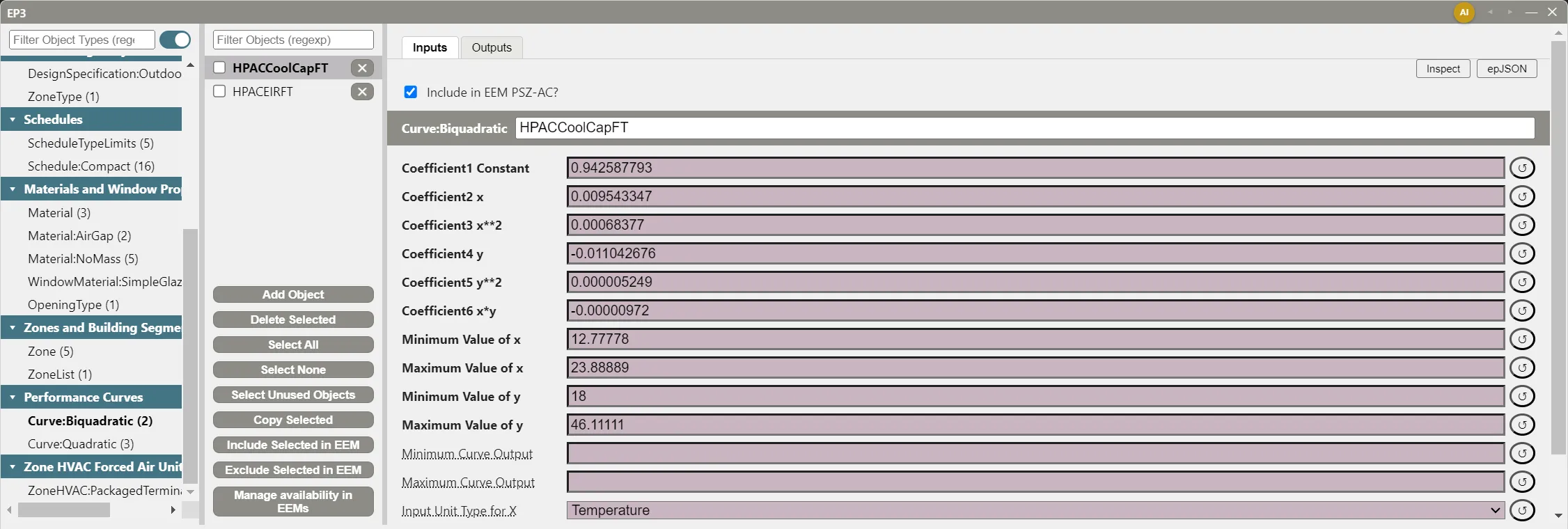
The PSZ-AC system template gives its DX cooling coil these two Curve:Biquadratic temperature curves (x = entering wet-bulb, y = condenser entering dry-bulb, both °C):
| Coefficient | HPACCoolCapFT (CAPFT) |
HPACEIRFT (EIRFT) |
|---|---|---|
| Coefficient1 Constant | 0.942587793 | 0.342414409 |
| Coefficient2 x | 0.009543347 | 0.034885008 |
| Coefficient3 x**2 | 0.00068377 | −0.0006237 |
| Coefficient4 y | −0.011042676 | 0.004977216 |
| Coefficient5 y**2 | 0.000005249 | 0.000437951 |
| Coefficient6 x*y | −0.00000972 | −0.000728028 |
| Range of x | 12.78 to 23.89 °C (55 to 75 °F) | 12.78 to 23.89 °C (55 to 75 °F) |
| Range of y | 18.0 to 46.11 °C (64.4 to 115 °F) | 18.0 to 46.11 °C (64.4 to 115 °F) |
The coil’s Gross Rated Cooling COP is 3.0. Take a coil sized to 10.55 kW (36,000 Btu/h, 3 tons).
At the rating point, x = 19.44 °C and y = 35.0 °C. Term by term:
CAPFT = 0.9426 + 0.1856 + 0.2585 − 0.3865 + 0.0064 − 0.0066 = 1.000
EIRFT = 0.3424 + 0.6783 − 0.2358 + 0.1742 + 0.5365 − 0.4955 = 1.000
So the coil delivers 10.55 kW × 1.000 = 10.55 kW and draws 10.55 kW × 1.000 / 3.0 = 3.52 kW. In IP units, the conditions are 67 °F wet-bulb and 95 °F outdoor, which the curves receive as 19.44 °C and 35.0 °C, so the multipliers are the same: the coil delivers 36,000 Btu/h at 3,518 W, an EER of 36,000 / 3,518 = 10.2 Btu/h per W, which is COP 3.0 × 3.412.
The flow-fraction curves check the same way at FF = 1.0: HPACCoolCapFFF = 0.8 + 0.2 = 1.000 and HPACEIRFFF = 1.1552 − 0.1808 + 0.0256 = 1.000.
A curve that does not come to 1.0 at its rating point shifts every timestep’s capacity or power by that factor, so evaluating a curve at its rating point is the first check on any curve you enter or receive.
2.3 What a curve’s inputs mean
A curve object does not say what its inputs are. A Curve:Biquadratic has an x and a y, and its Input Unit Type for X and Input Unit Type for Y fields say only what kind of quantity each is (Temperature, Dimensionless, and so on). The equipment field that references the curve defines which temperature or flow fraction x and y stand for, and EnergyPlus documents that in the field’s description; hovering over the field’s label in EP3 shows the same description. The same curve placed in a field it was not fitted for evaluates without error and returns a number with no meaning.
Coefficients are fitted to SI inputs. A curve’s coefficients and its minimum and maximum values are shown and entered in SI units in both SI and IP display, and the unit type fields do not convert them. To evaluate a curve at an IP condition, convert the condition to SI first, as in §2.2.
3. Curve and table forms
The coefficient field labels spell out each term (“Coefficient3 x**2”, “Coefficient6 x*y”), so a curve’s form can be read from its field list. The common forms:
| Curve type | Equation | Inputs | Typical use |
|---|---|---|---|
Curve:Linear |
C1 + C2·x | 1 | Simple proportional relationships |
Curve:Quadratic |
C1 + C2·x + C3·x² | 1 | Part-load fraction, chiller EIR vs. part-load ratio, boiler efficiency, flow-fraction modifiers |
Curve:Cubic |
C1 + C2·x + C3·x² + C4·x³ | 1 | DX heating capacity and EIR vs. outdoor temperature |
Curve:Biquadratic |
C1 + C2·x + C3·x² + C4·y + C5·y² + C6·x·y | 2 | DX coil and chiller capacity and EIR vs. two temperatures |
Curve:Bicubic |
the biquadratic terms + C7·x³ + C8·y³ + C9·x²·y + C10·x·y² | 2 | Higher-order two-variable fits |
Curve:QuadraticLinear |
(C1 + C2·x + C3·x²) + (C4 + C5·x + C6·x²)·y | 2 | Fits quadratic in x and linear in y |
EP3 also lists Curve:Quartic, Curve:Exponent, Curve:ExponentialDecay, Curve:ExponentialSkewNormal, Curve:Sigmoid, Curve:RectangularHyperbola1, Curve:RectangularHyperbola2, Curve:FanPressureRise, Curve:Functional:PressureDrop, Curve:DoubleExponentialDecay, Curve:CubicLinear, Curve:Triquadratic, Curve:ChillerPartLoadWithLift, Curve:QuadLinear, and Curve:QuintLinear, each used by particular equipment. Every EnergyPlus curve type is available in EP3.
The tables are Table:Lookup, Table:IndependentVariableList, and Table:IndependentVariable (§8).
4. Curves and tables in EP3
4.1 Finding and editing a curve
Curves and tables are edited in the main object dialog (EP3 in the top toolbar). Column 1 lists them in two groups, Performance Curves and Performance Tables; select a type such as Curve:Biquadratic, then a curve in Column 2, and its fields appear in Column 3 (The EP3 Interface and Model Settings).
Both groups appear only in complex view. Simplified view, which a model built with the Model Wizard starts in, leaves curves and tables out of Column 1; switch views with the view button in the top toolbar (The EP3 Interface and Model Settings).
A curve’s fields are its coefficients, Minimum Value of x and Maximum Value of x (and of y, z, and so on for multi-variable forms), the optional Minimum Curve Output and Maximum Curve Output, and the unit type fields. The coefficients and the input minimums and maximums are required, so their labels are bold.
4.2 How equipment points at a curve
Equipment refers to a curve by a field whose label ends in “Curve Name”, such as Total Cooling Capacity Function of Temperature Curve Name. The field is a dropdown of the curves and tables that have the number of inputs the field expects: a one-input field lists Curve:Linear, Curve:Quadratic, Curve:Cubic, and the other one-variable curves; a two-input field lists Curve:Biquadratic, Curve:Bicubic, Curve:QuadraticLinear, and the other two-variable curves. Both list every Table:Lookup. The curve fields of a zone unit’s coil are on the coil’s tab of the unit’s dialog (Zone-Level HVAC Equipment and Zone Sizing); a chiller’s or boiler’s are in its Selected Object dialog.
A curve field has no → button. To open the curve, select its type in the main object dialog’s Column 1 and type its name in Column 2’s Filter Objects box.
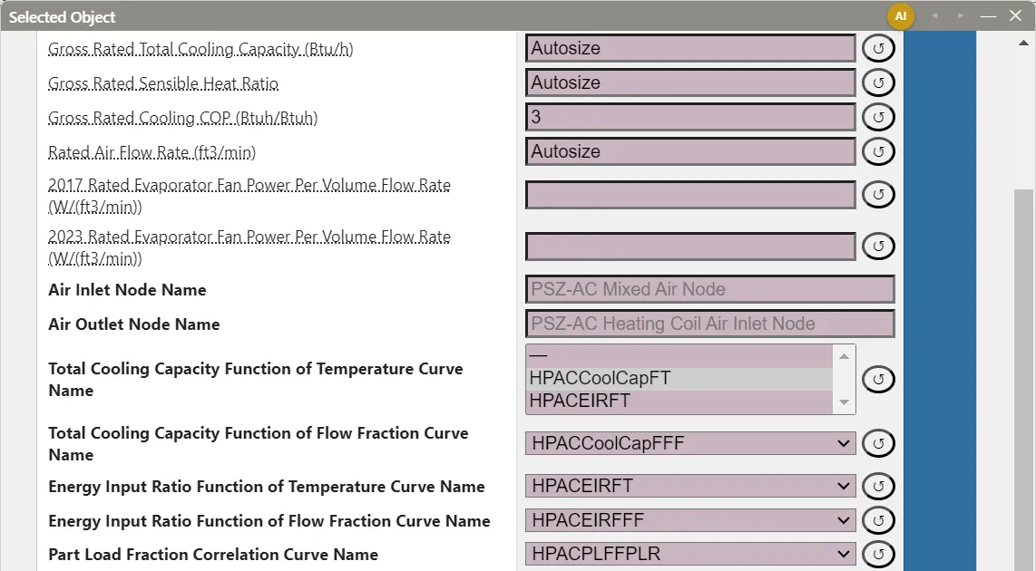
A curve is a separate, shared object. Several units can reference the same curve, and editing it changes all of them. To change one unit’s curve without affecting the others, check the curve in Column 2, click Copy Selected, rename and edit the copy, and select the copy in that unit’s curve field.
Curves follow the usual EEM rules (Energy Efficiency Measures (EEMs)): a coefficient entered while an EEM is active applies to that EEM, and a unit’s curve field can select a different curve in an EEM, which leaves the shared curve unchanged for every other unit.
A curve that equipment still references cannot be deleted. Delete Selected skips it, and its status message names the objects that reference it. Select Unused Objects checks the curves nothing references, for example after equipment has been replaced (The EP3 Interface and Model Settings).
EnergyPlus requires a curve’s name to be unique across all curve types and Table:Lookup, because a curve field names a curve without its type. EP3 keeps every Curve:*, Table:Lookup, Table:IndependentVariableList, and Table:IndependentVariable in one name namespace: a curve or table created, renamed, copied, or imported with a name another curve or table already has takes a numbered suffix instead (a rename to a taken name becomes <name> 2). When a model saved before this rule is opened, each curve or table whose name another type already uses is renamed <name> 1, <name> 2, and so on; the first in the model keeps the name.
4.3 Where a model’s curves come from
HVAC templates. Each library HVAC template carries the curves its equipment uses, and they come into the model with the system, from the Model Wizard or from the Import dialog’s templates (The HVAC Outliner and Creating HVAC Systems). The PSZ-AC template brings HPACCoolCapFT, HPACEIRFT, HPACCoolCapFFF, HPACEIRFFF, and HPACPLFFPLR. The PTHP template brings the same cooling curves plus its heating coil’s HPACHeatCapFT, HPACHeatEIRFT, HPACHeatCapFFF, HPACHeatEIRFFF, and HPACCOOLPLFFPLR. The Fan Coil template brings its chiller’s Main Chiller RecipCapFT, Main Chiller RecipEIRFT, and Main Chiller RecipEIRFPLR and its boiler’s Main Boiler Efficiency Curve. These are generic curves, not fits to a particular manufacturer’s product. When a template brings a curve with a name the model already has, the import’s same-name setting decides whether the existing curve is kept, overwritten, or joined by a renamed copy. A template you save yourself includes the curves its equipment uses (The HVAC Outliner and Creating HVAC Systems).
New coils. A new DX coil (single-speed, two-speed, two-stage, multispeed, and variable-speed DX cooling coils, Coil:Cooling:DX, and single-speed, multispeed, and variable-speed DX heating coils), water-to-air heat pump coil, heat pump water heater coil, multistage gas or electric heating coil, VRF coil, or VRF outdoor unit starts with default curves taken from the EnergyPlus example files. This applies whether the coil is added with a unit, added on its own, or chosen in a unit’s coil Type row. The default curves are named after the example curve and the coil class, such as WindACCoolCapFT (Coil:Cooling:DX:SingleSpeed default), and every new coil of that class shares them. The single-speed DX cooling defaults have the same coefficients as the PSZ-AC template’s curves in §2.2. A new ElectricEquipment:ITE:AirCooled object likewise starts with five curves from the EnergyPlus data center examples.
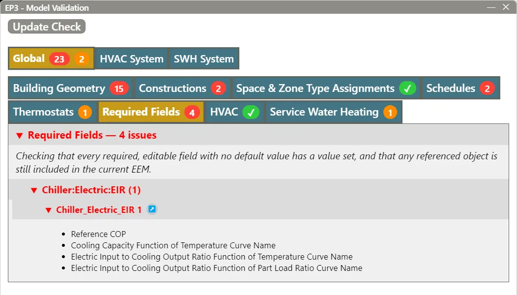
Other equipment. A chiller, boiler, or other component added with Add HVAC Component starts with its curve fields blank. Fill each required one before simulating; Model Validation lists the ones left blank (§9).
Imported files. An imported EnergyPlus file’s curves and tables are imported with the rest of the file, under the same same-name rules (Importing EnergyPlus Files). A file curve or table whose name another curve or table type already uses, in the model or in the same file, is imported as <name> 1 (or the next free number) whatever the same-name setting, and the fields that reference it follow the new name (§4.2).
5. The valid input range
Every curve has a Minimum Value of x and Maximum Value of x, and the same pair for each further input. They record the range of conditions the coefficients were fitted to. EnergyPlus replaces an input below the minimum with the minimum and an input above the maximum with the maximum before it evaluates the equation, and it issues no warning when it does. The polynomial is never extrapolated: the curve returns its boundary value for any condition past the boundary, however far past.
The limits do not stop the equipment. Whether a unit runs at a condition is set by fields on the equipment. A DX cooling coil’s Minimum Outdoor Dry-Bulb Temperature for Compressor Operation (default −25 °C, −13 °F) shuts its compressor off below that outdoor temperature, whatever its curves say; above it, the coil runs at its curves’ boundary performance whenever conditions are outside their range.
The limits protect the results only when they match the source data. Widening them, by copying a curve’s coefficients from one source without its range or by entering a generous range on the assumption that wider is more general, makes EnergyPlus evaluate the polynomial at conditions the data never covered.
5.1 Worked example: a 50 °C day
Take the coil of §2.2 on a 50 °C (122 °F) design day, with 19.44 °C (67 °F) entering wet-bulb. The curves were fitted only up to 46.11 °C (115 °F).
As entered, EnergyPlus evaluates both curves at y = 46.11 °C:
- CAPFT = 0.9426 + 0.1856 + 0.2585 − 0.5092 + 0.0112 − 0.0087 = 0.880, so capacity = 10.55 kW × 0.880 = 9.28 kW
- EIRFT = 1.293, so power = 9.28 kW × 1.293 / 3.0 = 4.00 kW
If Maximum Value of y had been widened to 50 °C or more, EnergyPlus would evaluate the polynomials at y = 50 °C:
- CAPFT = 0.838, so capacity = 10.55 kW × 0.838 = 8.84 kW
- EIRFT = 1.421, so power = 8.84 kW × 1.421 / 3.0 = 4.19 kW
In IP units: 36,000 Btu/h × 0.880 = 31,680 Btu/h at 4,001 W (EER 7.9) as entered, against 36,000 Btu/h × 0.838 = 30,180 Btu/h at 4,189 W (EER 7.2) with the widened range. The two differ by 5% in capacity and 4.5% in power, and neither is backed by data: the clamped result holds the 46.11 °C performance constant, and the extrapolated one follows a polynomial past its data. For conditions beyond 46.11 °C, use manufacturer data that covers them, and in every case enter limits that match the data the curve was fitted to.
6. Limiting the output: Minimum and Maximum Curve Output
Minimum Curve Output and Maximum Curve Output limit the curve’s result after it is evaluated, independently of the input limits. EnergyPlus replaces a result below the minimum with the minimum and above the maximum with the maximum, again without a warning. Left blank, they impose no limit.
They matter for curves whose output has a physical bound that the fit does not guarantee. A quadratic fitted through a few points can dip, inside its input range, to a value the equipment cannot have, such as a negative capacity multiplier. A Minimum Curve Output keeps the result above that bound wherever in the range the fit misbehaves.
7. Part-load behavior
7.1 Part load fraction for cycling equipment
Single-speed DX equipment meets a part load by cycling its compressor on and off, and each cycle loses some efficiency while the coil comes up to temperature. The Part Load Fraction Correlation Curve Name curve gives the part-load fraction (PLF) as a function of the part-load ratio (PLR), and EnergyPlus runs the coil for a runtime fraction of PLR / PLF of the timestep. The curve should equal 1.0 at PLR = 1.0. For PLR below 1.0, PLF must be at least 0.7 and at least PLR: EnergyPlus resets a PLF below 0.7 to 0.7 with a warning, and where PLF is below PLR it warns and limits the runtime fraction to 1.0. EnergyPlus gives PLF = 0.85 + 0.15·PLR as typical for a single-speed DX cooling coil, and that is the PSZ-AC template’s HPACPLFFPLR.
Worked example: the coil of §2.2 at the rating temperatures, meeting a load of 40% of its capacity:
- PLF = 0.85 + 0.15 × 0.4 = 0.91
- Runtime fraction = 0.4 / 0.91 = 0.440
- Cooling delivered = 0.4 × 10.55 kW = 4.22 kW (14,400 Btu/h)
- Power = 3.52 kW × 0.440 = 1.55 kW, against 3.52 kW × 0.4 = 1.41 kW with no cycling loss: 1 / 0.91 = 1.10, or 10% more
In IP units the part-load EER is 14,400 Btu/h / 1,546 W = 9.3, against 10.2 at full load. A PLF curve equal to 1.0 at every PLR (Coefficient1 Constant 1, the other coefficients 0) models no cycling loss.
7.2 Part-load EIR for chillers
A Chiller:Electric:EIR computes its power as available capacity × (1 / Reference COP) × EIRFT × EIRFPLR, where EIRFPLR is the curve named in Electric Input to Cooling Output Ratio Function of Part Load Ratio Curve Name. EIRFPLR is power as a fraction of full-load power at the same temperatures; it equals 1.0 at PLR = 1.0 and falls toward 0 as PLR falls.
Worked example: the Fan Coil template’s chiller has a Reference COP of 3.2, a Reference Leaving Chilled Water Temperature of 6.67 °C (44 °F), and a Reference Entering Condenser Fluid Temperature of 29.4 °C (85 °F). At those temperatures its Main Chiller RecipCapFT evaluates to 0.998 and Main Chiller RecipEIRFT to 1.000, close to the 1.0 normalization. Its part-load curve is Main Chiller RecipEIRFPLR = 0.088065 + 1.137742·PLR − 0.225806·PLR²:
- At PLR = 1.0: 0.088065 + 1.137742 − 0.225806 = 1.000
- At PLR = 0.5: 0.088065 + 0.568871 − 0.056452 = 0.600
At half load the chiller draws 60% of its full-load power to deliver 50% of its capacity, so its power per unit of cooling rises by 0.600 / 0.5 = 1.20. Its COP falls from 3.2 to 3.2 / 1.20 = 2.66; in IP units, from 3.517 / 3.2 = 1.10 kW/ton to 1.10 × 1.20 = 1.32 kW/ton.
The same curves set the chiller’s range: x (leaving chilled water) 5 to 10 °C (41 to 50 °F) and y (entering condenser fluid) 24 to 35 °C (75.2 to 95 °F). Condenser water colder than 24 °C is evaluated as 24 °C (§5). Central Plant Equipment and Plant Loops covers the chiller’s other fields.
7.3 Boiler efficiency
A Boiler:HotWater’s Normalized Boiler Efficiency Curve Name curve multiplies its Nominal Thermal Efficiency. With a one-input curve, the input is the part-load ratio; with a two-input curve, x is the part-load ratio and y the boiler water temperature chosen by Efficiency Curve Temperature Evaluation Variable.
The Fan Coil template’s Main Boiler Efficiency Curve is 0.97 + 0.0633·PLR − 0.0333·PLR², with a Nominal Thermal Efficiency of 0.80. At PLR = 1.0 it equals 0.97 + 0.0633 − 0.0333 = 1.000, an efficiency of 0.80; at PLR = 0.25 it equals 0.97 + 0.0158 − 0.0021 = 0.984, an efficiency of 0.80 × 0.984 = 0.787.
7.4 Coefficients entered on the equipment
Some equipment takes its part-load polynomial as coefficient fields on the equipment object instead of a curve reference: Fan:VariableVolume’s fan power coefficients (Fans and Fan Power) and Pump:VariableSpeed’s part-load coefficients (Central Plant Equipment and Plant Loops). The same normalization applies: the polynomial should equal 1.0 at full flow.
8. Performance tables
A performance table represents the same kind of relationship as a curve, with tabulated data in place of an equation. It suits data that a low-order polynomial fits poorly, or catalog data used as published. A table takes three kinds of object, each in the Performance Tables group:
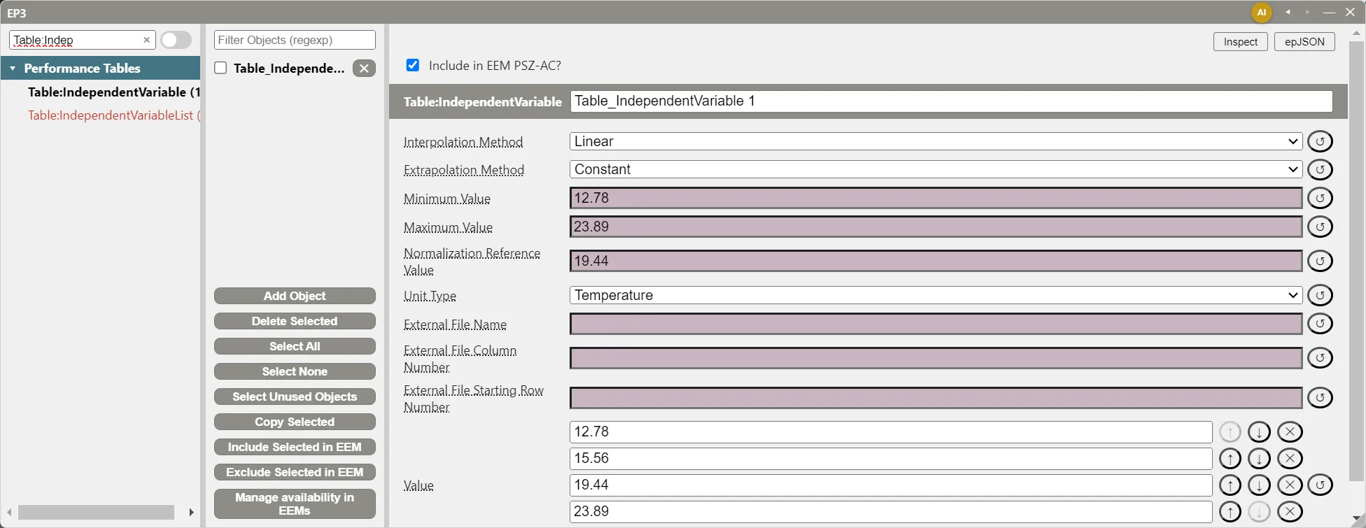
Table:IndependentVariable— one input’s values, entered in its Value list (+ Add adds a value; ↑, ↓, and ✕ reorder or remove one), with its Interpolation Method (Linear or Cubic, between values), Extrapolation Method (Constant or Linear, beyond the first and last value), optional Minimum Value and Maximum Value, Normalization Reference Value, and Unit Type.Table:IndependentVariableList— the inputs, in order, each chosen from the model’sTable:IndependentVariableobjects.Table:Lookup— the Independent Variable List Name, the Output Value list, Normalization Method and Normalization Divisor, and optional Minimum Output and Maximum Output.
Equipment references the Table:Lookup. Its output values are ordered with the last input varying fastest. In place of typed values, the variables and the table can read their data from a CSV file through External File Name, External File Column Number, and External File Starting Row Number.
Tables make the extrapolation choice explicit. With Extrapolation Method Constant, a table holds its boundary value, as a curve does. With Linear, it extends the trend at the boundary out to the variable’s Minimum Value or Maximum Value, and beyond those holds the value with a warning. Linear extrapolation extends the data on purpose; choose it only where the trend beyond the data is known.
Normalization turns catalog data in kW or Btu/h into the fraction-of-rated form equipment expects. Enter the rating condition in each variable’s Normalization Reference Value and set the table’s Normalization Method to AutomaticWithDivisor; EnergyPlus divides the output values by the table’s value at those reference values, so the table equals 1.0 at the rating point. DivisorOnly divides by Normalization Divisor alone. Either every variable in a list has a Normalization Reference Value or none does.
9. Checking curves
EP3 does not plot curves. To see a curve’s shape, evaluate it, by hand or in a spreadsheet, at its rating point (it should be 1.0, as in §2.2), at the corners of its input range, and at the conditions the model will reach, and compare the results with the source data.
Model Validation. The Validate button’s Required Fields tab lists every required field left blank. That covers a curve’s coefficients and input limits, an equipment’s required curve fields, and a curve field that references a curve not included in the EEM being checked (Model Troubleshooting and Quality Assurance). Validation does not check a curve’s values: its normalization, its range, or whether its inputs suit the field that uses it.
An Object Names tab appears only when two curves or tables of different types in the checked EEM share a name. Its Curve & Table Names check lists each clash as a warning, with the name the curve is exported under until you rename it.
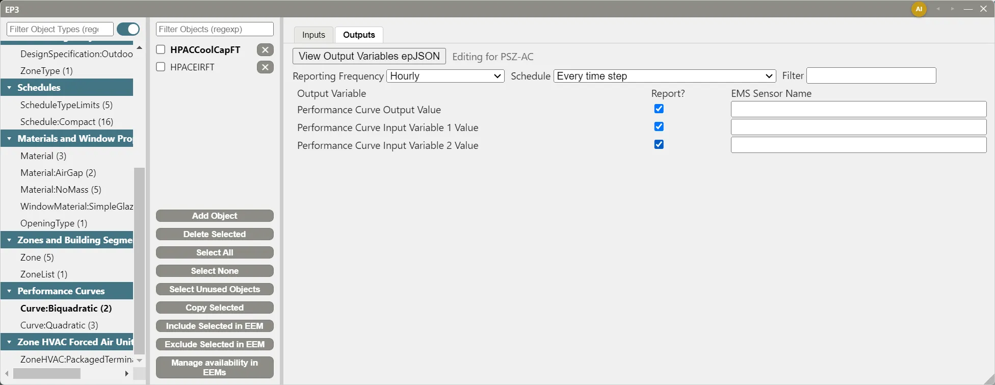
Curve output variables. A curve’s or table’s Outputs tab, beside Inputs in the main object dialog, requests Performance Curve Output Value and Performance Curve Input Variable 1 Value, Input Variable 2 Value, and so on. After a run, plotting the inputs against the curve’s range shows how often and how far the model operates outside the fitted data, and the output shows the multiplier applied (Running Simulations).
Atlas, EP3’s AI assistant, also works with curves; The EP3 AI Assistant covers what it can and cannot do with them.
10. Where to Look Next
- Central Plant Equipment and Plant Loops — the chillers, boilers, heat pumps, towers, and pumps whose curve fields this chapter explains.
- Zone-Level HVAC Equipment and Zone Sizing — the zone units whose coil tabs hold DX curve fields.
- Fans and Fan Power — fan power at part flow.
- Energy Efficiency Measures (EEMs) — changing curves or curve assignments in an efficiency measure.
- Importing EnergyPlus Files — bringing in curves and tables from another model.
- Input Output Reference: Group – Performance Curves and Input Output Reference:
Table:Lookup— every curve and table type, field by field. - Engineering Reference: Performance Curves — the equations, and how a biquadratic is fitted to normalized catalog data.
This handbook is also built into EP3 (Help), where its EnergyPlus links open the EnergyPlus Reference. Technical specifications · Book a demo